Algorithms for prediction

Part 1 of 2: Penalized Linear Regression

Problem Set 1: Discussion

Term	Meaning
Unit of analysis	A row of your data
Unit-specific quantity	Outcome or potential outcome(s)
Target population	Set of units over which to aggregate

Why? To ask $\hat{Y}$ questions, not $\hat\beta$ questions

Problem Set 1: Discussion

Some language notes:

Causal language
- X verb Y
Non-causal language
- differences in Y across X

Problem Set 1: Discussion

Many submitted models like this:

\[E(Y \mid X) = \alpha + \beta X\]

When $X$ is binary, this model is like taking subgroup means.

\[ \begin{aligned} E(Y\mid X = 0) &= \alpha \\ E(Y\mid X = 1) &= \alpha + \beta \end{aligned} \]

It is not really a “model” at all

Problem Set 1: Discussion

Other things to discuss?

Goals for today

review OLS to predict
understand regularization to estimate
many parameters while avoiding high variance
walk through three regularized linear model algorithms
- multilevel models
- ridge regression
- LASSO regression

Data

Data: Baseball salaries

All 944 Major League Baseball Players, Opening Day 2023.
Compiled by USA Today
I appended each team’s win-loss record from 2022
Available in baseball_population.csv

Data: Baseball salaries

Load packages:

library(tidyverse)
library(scales)
library(foreach)

Load data:

baseball_population <- read_csv(
  "https://ilundberg.github.io/soc212b/data/baseball_population.csv"
)

Data: Baseball salaries

baseball_population |> print(n = 3)

# A tibble: 944 × 5
  player               salary position team    team_past_record
  <chr>                 <dbl> <chr>    <chr>              <dbl>
1 Bumgarner, Madison 21882892 LHP      Arizona            0.457
2 Marte, Ketel       11600000 2B       Arizona            0.457
3 Ahmed, Nick        10375000 SS       Arizona            0.457
# ℹ 941 more rows

Data: Baseball salaries

Code

baseball_population |>
  group_by(position) |>
  summarize(salary = mean(salary)) |>
  mutate(position = fct_reorder(position, -salary)) |>
  ggplot(aes(x = position, y = salary)) +
  geom_bar(stat = "identity") +
  geom_text(
    aes(
      label = label_currency(
        scale = 1e-6, accuracy = .1, suffix = " m"
      )(salary)
    ), 
    y = 0, color = "white", fontface = "bold",
    vjust = -1
  ) +
  scale_y_continuous(
    name = "Average Salary",
    labels = label_currency(scale = 1e-6, accuracy = 1, suffix = " million")
  ) +
  scale_x_discrete(
    name = "Position",
    labels = function(x) {
      case_when(
        x == "C" ~ "C\nCatcher",
        x == "RHP" ~ "RHP\nRight-\nHanded\nPitcher",
        x == "LHP" ~ "LHP\nLeft-\nHanded\nPitcher",
        x == "1B" ~ "1B\nFirst\nBase",
        x == "2B" ~ "2B\nSecond\nBase",
        x == "SS" ~ "SS\nShortstop",
        x == "3B" ~ "3B\nThird\nBase",
        x == "OF" ~ "OF\nOutfielder",
        x == "DH" ~ "DH\nDesignated\nHitter"
      )
    }
  ) +
  theme_minimal() +
  theme(text = element_text(size = 18)) +
  ggtitle("Baseball salaries vary across positions")

Data: Baseball salaries

Code

baseball_population |>
  group_by(team) |>
  summarize(
    salary = mean(salary),
    team_past_record = unique(team_past_record)
  ) |>
  ggplot(aes(x = team_past_record, y = salary)) +
  geom_point() +
  ggrepel::geom_text_repel(
    aes(label = team),
    size = 2
  ) +
  scale_x_continuous(
    name = "Team Past Record: Proportion Wins in 2022"
  ) +
  scale_y_continuous(
    name = "Team Average Salary in 2023",
    labels = label_currency(
      scale = 1e-6, 
      accuracy = 1, 
      suffix = " million"
    )
  ) +
  theme_minimal() +
  theme(text = element_text(size = 18)) +
  ggtitle("Baseball salaries vary across teams")

Task

Task: Predict Dodger mean salary

We have the full population:

true_dodger_mean <- baseball_population |>
  # Restrict to the Dodgers
  filter(team == "L.A. Dodgers") |>
  # Record the mean salary
  summarize(mean_salary = mean(salary)) |>
  # Pull that estimate out of the data frame to just be a number
  pull(mean_salary)

The true Dodger mean salary on Opening Day 2023 was $6,232,196.

Task: Predict Dodger mean salary

Imagine we have

predictors for everyone
salary for a sample of 5 players per team

Task: Predict Dodger mean salary

learn model on everyone
create data to predict: the Dodger population
predict the outcome in this target population
average over units

Task: Predict Dodger mean salary

Draw a sample of 5 players per team.

baseball_sample <- baseball_population |>
  group_by(team) |>
  slice_sample(n = 5) |>
  ungroup() |>
  print()

# A tibble: 150 × 5
   player                 salary position team    team_past_record
   <chr>                   <dbl> <chr>    <chr>              <dbl>
 1 Carroll, Corbin       1625000 OF       Arizona            0.457
 2 Herrera, Jose          724300 C        Arizona            0.457
 3 Melancon, Mark*       6000000 RHP      Arizona            0.457
 4 Ahmed, Nick          10375000 SS       Arizona            0.457
 5 Robinson, Kristian**   720000 OF       Arizona            0.457
 6 Arcia, Orlando        2300000 SS       Atlanta            0.623
 7 Lee, Dylan             730000 LHP      Atlanta            0.623
 8 Pillar, Kevin         3000000 OF       Atlanta            0.623
 9 Matzek, Tyler*        1200000 LHP      Atlanta            0.623
10 Hilliard, Sam          750000 OF       Atlanta            0.623
# ℹ 140 more rows

Task: Predict Dodger mean salary

Our 5 sampled Dodger players have an average salary of $7,936,238.

# A tibble: 5 × 5
  player           salary position team         team_past_record
  <chr>             <dbl> <chr>    <chr>                   <dbl>
1 Phillips, Evan  1300000 RHP      L.A. Dodgers            0.685
2 Miller, Shelby  1500000 RHP      L.A. Dodgers            0.685
3 Taylor, Chris  15000000 OF       L.A. Dodgers            0.685
4 Betts, Mookie  21158692 OF       L.A. Dodgers            0.685
5 Outman, James    722500 OF       L.A. Dodgers            0.685

Task: Create data to predict

We want to predict salary for all Dodger players:

dodgers_to_predict <- baseball_population |>
  filter(team == "L.A. Dodgers") |>
  select(-salary)

OLS

Ordinary Least Squares: Model

Model salary as a function of team_past_record

ols <- lm(
  salary ~ team_past_record,
  data = baseball_sample
)

Ordinary Least Squares: Predict

ols_predicted <- dodgers_to_predict |>
  mutate(predicted_salary = predict(ols, newdata = dodgers_to_predict)) |>
  print(n = 3)

# A tibble: 35 × 5
  player           position team         team_past_record predicted_salary
  <chr>            <chr>    <chr>                   <dbl>            <dbl>
1 Freeman, Freddie 1B       L.A. Dodgers            0.685         5552999.
2 Heyward, Jason   OF       L.A. Dodgers            0.685         5552999.
3 Betts, Mookie    OF       L.A. Dodgers            0.685         5552999.
# ℹ 32 more rows

Ordinary Least Squares: Average

Average predictions over the target population

ols_estimate <- ols_predicted |>
  summarize(ols_estimate = mean(predicted_salary)) |>
  print()

# A tibble: 1 × 1
  ols_estimate
         <dbl>
1     5552999.

Performance of OLS

We usually have only one sample
In this case, we have the population

Plan
- draw repeated samples
- evaluate performance over repeated samples

Performance of OLS: Estimator function

A function that

takes in a sample
returns an estimate

Performance of OLS: Estimator function

ols_estimator <- function(
    sample = baseball_sample, 
    to_predict = dodgers_to_predict
) {
  # Learn a model in the sample
  ols <- lm(
    salary ~ team_past_record,
    data = sample
  )
  # Predict for our target population
  ols_predicted <- to_predict |>
    mutate(predicted_salary = predict(ols, newdata = to_predict))
  # Average over the target population
  ols_estimate_star <- ols_predicted |>
    summarize(ols_estimate = mean(predicted_salary)) |>
    pull(ols_estimate)
  # Return the estimate
  return(ols_estimate_star)
}

Performance of OLS: Estimator function

Apply the estimator in repeated samples.

Code

many_sample_estimates <- foreach(
  repetition = 1:100, .combine = "c"
) %do% {
  # Draw a sample from the population
  baseball_sample <- baseball_population |>
    group_by(team) |>
    slice_sample(n = 5) |>
    ungroup()
  # Apply the estimator to the sample
  estimate <- ols_estimator(baseball_sample)
  return(estimate)
}

Performance of OLS: Estimator function

Code

tibble(y = many_sample_estimates) |>
  # Random jitter for x
  mutate(x = runif(n(), -.1, .1)) |>
  ggplot(aes(x = x, y = many_sample_estimates)) +
  geom_point() +
  scale_y_continuous(
    name = "Dodger Mean Salary",
    labels = label_millions
  ) +
  theme_minimal() +
  theme(text = element_text(size = 18)) +
  scale_x_continuous(
    breaks = NULL, limits = c(-.5,.5),
    name = "Each dot is an OLS estimate\nin one sample from the population"
  ) +
  geom_hline(yintercept = true_dodger_mean, linetype = "dashed") +
  annotate(geom = "text", x = -.5, y = true_dodger_mean, hjust = 0, vjust = -.5, label = "True mean in\nDodger subpopulation", size = 3)

Approximation Error

Model approximation error

Code

population_ols <- lm(salary ~ team_past_record, data = baseball_population)
forplot <- baseball_population |>
  mutate(fitted = predict(population_ols)) |>
  group_by(team) |>
  summarize(
    truth = mean(salary),
    fitted = unique(fitted),
    team_past_record = unique(team_past_record)
  )
forplot_dodgers <- forplot |> filter(team == "L.A. Dodgers")
forplot |>
  ggplot(aes(x = team_past_record)) +
  geom_point(aes(y = truth, color = team == "L.A. Dodgers")) +
  geom_line(aes(y = fitted)) +
  geom_segment(
    data = forplot_dodgers,
    aes(
      yend = fitted - 3e5, y = truth + 3e5,
    ), 
    arrow = arrow(length = unit(.05,"in"), ends = "both"), color = "dodgerblue"
  ) +
  geom_text(
    data = forplot_dodgers,
    aes(
      x = team_past_record + .02, 
      y = .5 * (fitted + truth), 
      label = "model\napproximation\nerror"
    ),
    size = 2, color = "dodgerblue", hjust = 0
  ) +
  geom_text(
    data = forplot_dodgers, 
    aes(y = truth, label = "L.A.\nDodgers"),
    color = "dodgerblue",
    vjust = 1.8, size = 2
  ) +
  scale_color_manual(
    values = c("gray","dodgerblue")
  ) +
  scale_y_continuous(
    name = "Team Mean Salary in 2023", 
    labels = label_currency(
      scale = 1e-6, accuracy = .1, suffix = " million"
    )
  ) +
  scale_x_continuous(limits = c(.3,.8), name = "Team Past Record: Proportion Wins in 2022") +
  theme_classic() +
  theme(legend.position = "none", text = element_text(size = 18))

Model approximation error

How to solve model approximation error?

A model with more parameters

ols_team_categories <- lm(
  salary ~ team,
  data = baseball_sample
)

OLS with many parameters

Code

# Create many sample estimates with categorical teams
many_sample_estimates_categories <- foreach(
  repetition = 1:100, .combine = "c"
) %do% {
  # Draw a sample from the population
  baseball_sample <- baseball_population |>
    group_by(team) |>
    slice_sample(n = 5) |>
    ungroup()
  # Apply the estimator to the sample# Learn a model in the sample
  ols <- lm(
    salary ~ team,
    data = baseball_sample
  )
  # Predict for our target population
  ols_predicted <- dodgers_to_predict |>
    mutate(predicted_salary = predict(ols, newdata = dodgers_to_predict))
  # Average over the target population
  ols_estimate <- ols_predicted |>
    summarize(ols_estimate = mean(predicted_salary)) |>
    pull(ols_estimate)
  # Return the estimate
  return(ols_estimate)
}
# Visualize
tibble(x = "OLS linear in\nteam past record", y = many_sample_estimates) |>
  bind_rows(
    tibble(x = "OLS with categorical\nteam indicators", y = many_sample_estimates_categories)
  ) |>
  ggplot(aes(x = x, y = y)) +
  geom_jitter(width = .2, height = 0) +
  scale_y_continuous(
    name = "Dodger Mean Salary", 
    labels = label_currency(
      scale = 1e-6, accuracy = .1, suffix = " million"
    )
  ) +
  theme_minimal() +
  theme(text = element_text(size = 18)) +
  scale_x_discrete(
    name = "Estimator"
  ) +
  ggtitle(NULL, subtitle = "Each dot is an estimate in one sample from the population") +
  geom_hline(yintercept = true_dodger_mean, linetype = "dashed") +
  annotate(geom = "text", x = .4, y = true_dodger_mean, hjust = 0, vjust = .5, label = "Truth in\npopulation", size = 3)

Regularization

Two estimators:

nonparametric mean of 5 sampled players on each team
(high variance)
linear prediction: linear fit on team past record
(biased by model approximation error)

We might regularize the nonparametric toward the linear prediction

Regularization

Code

estimates_by_w <- foreach(w_value = seq(0,1,.05), .combine = "rbind") %do% {
  tibble(
    w = w_value,
    estimate = (1 - w) * dodger_sample_mean + w * ols_estimate
  )
}
estimates_by_w |>
  ggplot(aes(x = w, y = estimate)) +
  geom_point() +
  geom_line() +
  geom_text(
    data = estimates_by_w |>
      filter(w %in% c(0,1)) |>
      mutate(
        w = w + c(1,-1) * .13, 
        hjust = c(0,1),
        label = c("Nonparametric Dodger Sample Mean",
                  "Linear Prediction from OLS")
      ),
    aes(label = label, hjust = hjust)
  ) +
  geom_segment(
     data = estimates_by_w |>
      filter(w %in% c(0,1)) |>
       mutate(x = w + c(1,-1) * .12,
              xend = w + c(1,-1) * .04),
     aes(x = x, xend = xend),
     arrow = arrow(length = unit(.08,"in"))
  ) +
  annotate(
    geom = "text", x = .3, y = estimates_by_w$estimate[12],
    label = "Partial\nPooling\nEstimates",
    vjust = 1
  ) +
  annotate(
    geom = "segment", 
    x = c(.3,.4), 
    xend = c(.3,.55),
    y = estimates_by_w$estimate[c(11,14)],
    yend = estimates_by_w$estimate[c(8,14)],
    arrow = arrow(length = unit(.08,"in"))
  ) +
  scale_x_continuous("Weight: Amount of Shrinkage Toward Linear Fit") +
  scale_y_continuous(
    labels = label_currency(
      scale = 1e-6, accuracy = .1, suffix = " million"
    ),
    name = "Dodger Mean Salary Estimates",
    expand = expansion(mult =.1)
  ) +
  theme_minimal() +
  theme(text = element_text(size = 18))

Regularization: How much?

Want to minimize expected squared error.

\[ \text{Expected Squared Error}(\hat\mu_\text{Dodgers}) = \text{E}_S\left(\left(\hat\mu_\text{Dodgers}(S) - \mu_\text{Dodgers}\right)^2\right) \]

Regularization: How much?

Code

repeated_simulations <- foreach(rep = 1:100, .combine = "rbind") %do% {
  
  a_sample <- baseball_population |>
    group_by(team) |>
    slice_sample(n = 5) |>
    ungroup()
  
  ols_fit <- lm(salary ~ team_past_record, data = a_sample)
  
  ols_estimate <- predict(
    ols_fit, 
    newdata = baseball_population |> 
      filter(team == "L.A. Dodgers") |>
      distinct(team_past_record)
  )
  
  nonparametric_estimate <- a_sample |>
    filter(team == "L.A. Dodgers") |>
    summarize(salary = mean(salary)) |>
    pull(salary)
  
  foreach(w_value = seq(0,1,.05), .combine = "rbind") %do% {
    tibble(
      w = w_value,
      estimate = w * ols_estimate + (1 - w) * nonparametric_estimate
    )
  }
}

aggregated <- repeated_simulations |>
  group_by(w) |>
  summarize(mse = mean((estimate - true_dodger_mean) ^ 2)) |>
  mutate(best = mse == min(mse))

aggregated |>
  ggplot(aes(x = w, y = mse, color = best)) +
  geom_line() +
  geom_point() +
  scale_y_continuous(name = "Expected Squared Error\nfor Dodger Mean Salary") +
  scale_x_continuous(name = "Weight: Amount of Shrinkage Toward Linear Fit") +
  scale_color_manual(values = c("black","dodgerblue")) +
  geom_vline(xintercept = c(0,1), linetype = "dashed") +
  theme_minimal() +
  theme(legend.position = "none", text = element_text(size = 18)) +
  annotate(
    geom = "text", 
    x = c(0.02,.98), 
    y = range(aggregated$mse),
    hjust = c(0,1), vjust = c(0,1),
    size = 3,
    label = c(
      "Nonparametric estimator:\nDodger mean salary",
      "Model-based estimator:\nOLS linear prediction"
    )
  ) +
  annotate(
    geom = "text", 
    x = aggregated$w[aggregated$best], 
    y = min(aggregated$mse) + .2 * diff(range(aggregated$mse)),
    vjust = -.1,
    label = "Best-Performing\nEstimator",
    size = 3,
    color = "dodgerblue"
  ) +
  annotate(
    geom = "segment",
    x = aggregated$w[aggregated$best], 
    y = min(aggregated$mse) + .18 * diff(range(aggregated$mse)),
    yend = min(aggregated$mse) + .05 * diff(range(aggregated$mse)),
    arrow = arrow(length = unit(.08,"in")),
    color = "dodgerblue"
  )

Multilevel models

Multilevel models: Idea

many groups
a few observations per group
partially pool between
- group-specific mean estimates (high variance)
- a model pooled across groups (potentially biased)

Multilevel models: Code

library(lme4)

multilevel <- lmer(
  salary ~ team_past_record + (1 | team), 
  data = baseball_sample
)

Make predictions

multilevel_predicted <- dodgers_to_predict |>
  mutate(
    fitted = predict(multilevel, newdata = dodgers_to_predict)
  )

Multilevel models: Intuition

Code

p <- baseball_sample |>
  group_by(team) |>
  mutate(nonparametric = mean(salary)) |>
  ungroup() |>
  mutate(
    fitted = predict(multilevel)
  ) |>
  distinct(team, team_past_record, fitted, nonparametric) |>
  ungroup() |>
  ggplot(aes(x = team_past_record)) +
  geom_point(aes(y = nonparametric)) +
  geom_abline(
    intercept = fixef(multilevel)[1], 
    slope = fixef(multilevel)[2], 
    linetype = "dashed"
  ) +
  geom_segment(
    aes(y = nonparametric, yend = fitted),
    arrow = arrow(length = unit(.05,"in"))
  ) +
  geom_point(aes(y = nonparametric)) +
  theme_minimal() +
  theme(text = element_text(size = 18)) +
  scale_y_continuous(
    name = "Team Mean Salary in 2023", 
    labels = label_currency(
      scale = 1e-6, accuracy = .1, suffix = " million"
    )
  ) +
  scale_x_continuous(name = "Team Past Record: Proportion Wins in 2022") +
  ggtitle("Multilevel model on a sample of 5 players per team",
          subtitle = "Points are nonparametric sample mean estimates.\nArrow ends are multilevel model estimates.\nDashed line is an unregularized fixed effect.")
p

Multilevel models: Intuition

Code

bigger_sample <- baseball_population |>
  group_by(team) |>
  slice_sample(n = 20) |>
  ungroup()
multilevel_big <- lmer(formula(multilevel), data = bigger_sample)
bigger_sample |>
  group_by(team) |>
  mutate(nonparametric = mean(salary)) |>
  ungroup() |>
  mutate(
    fitted = predict(multilevel_big)
  ) |>
  distinct(team, team_past_record, fitted, nonparametric) |>
  ungroup() |>
  ggplot(aes(x = team_past_record)) +
  geom_point(aes(y = nonparametric)) +
  geom_abline(
    intercept = fixef(multilevel_big)[1], 
    slope = fixef(multilevel_big)[2], 
    linetype = "dashed"
  ) +
  geom_segment(
    aes(y = nonparametric, yend = fitted),
    arrow = arrow(length = unit(.05,"in"))
  ) +
  geom_point(aes(y = nonparametric)) +
  #ggrepel::geom_text_repel(aes(y = fitted, label = team), size = 2) +
  theme_minimal() +
  theme(text = element_text(size = 18)) +
  scale_y_continuous(
    name = "Team Mean Salary in 2023", 
    labels = label_currency(
      scale = 1e-6, accuracy = .1, suffix = " million"
    ),
    limits = layer_scales(p)$y$range$range
  ) +
  scale_x_continuous(name = "Team Past Record: Proportion Wins in 2022") +
  ggtitle("Multilevel model on a sample of 20 players per team",
          subtitle = "Points are nonparametric sample mean estimates.\nArrow ends are multilevel model estimates.\nDashed line is an unregularized fixed effect.")

Multilevel models: Performance

Code

many_sample_estimates_multilevel <- foreach(
  repetition = 1:100, .combine = "c"
) %do% {
  # Draw a sample from the population
  baseball_sample <- baseball_population |>
    group_by(team) |>
    slice_sample(n = 5) |>
    ungroup()
  # Apply the estimator to the sample# Learn a model in the sample
  multilevel <- lmer(
    salary ~ team_past_record + (1 | team),
    data = baseball_sample
  )
  # Predict for our target population
  mutilevel_predicted <- dodgers_to_predict |>
    mutate(predicted_salary = predict(multilevel, newdata = dodgers_to_predict))
  # Average over the target population
  mutilevel_estimate <- mutilevel_predicted |>
    summarize(mutilevel_estimate = mean(predicted_salary)) |>
    pull(mutilevel_estimate)
  # Return the estimate
  return(mutilevel_estimate)
}
# Visualize
tibble(x = "OLS with\nlinear record", y = many_sample_estimates) |>
  bind_rows(
    tibble(x = "OLS with\nteam indicators", y = many_sample_estimates_categories)
  ) |>
  bind_rows(
    tibble(x = "Multilevel\nmodel", y = many_sample_estimates_multilevel)
  ) |>
  ggplot(aes(x = x, y = y)) +
  geom_jitter(width = .2, height = 0) +
  scale_y_continuous(
    name = "Dodger Mean Salary", 
    labels = label_currency(
      scale = 1e-6, accuracy = .1, suffix = " million"
    )
  ) +
  theme_minimal() +
  scale_x_discrete(
    name = "Estimator"
  ) +
  ggtitle(NULL, subtitle = "Each dot is an estimate in one sample from the population") +
  geom_hline(yintercept = true_dodger_mean, linetype = "dashed") +
  annotate(geom = "text", x = .4, y = true_dodger_mean, hjust = 0, vjust = .5, label = "Truth in\npopulation", size = 3)

Multilevel models: In math

Person-level model. For player $i$ on team $t$,

\[\begin{equation} Y_{ti} \sim \text{Normal}\left(\mu_t, \sigma^2\right) \end{equation}\]

Group-level model. There is a model for $\mu_t$, mean salary on team $t$.

\[\mu_t \sim \text{Normal}(\alpha + X_t\beta, \tau^2)\] where $X_t$ is team past record

Ridge regression

Often taught in data science classes

many coefficients
penalize large coefficients
minimize a loss function

Ridge regression

\[ Y_{ti} = \alpha + \beta X_t + \gamma_{t} + \epsilon_{ti} \]

Minimize a loss function:

\[ \underbrace{\sum_t\sum_i\left(Y_{ti} - \left(\alpha + \beta X_t + \gamma_{t}\right)\right)^2}_\text{Sum of Squared Error} + \underbrace{\lambda\sum_t\gamma_t^2}_\text{Penalty} \]

Ridge regression: Code

library(glmnet)

ridge <- glmnet(
  x = model.matrix(~ -1 + team_past_record + team, data = baseball_sample),
  y = baseball_sample$salary,
  penalty.factor = c(0,rep(1,30)),
  # Choose the ridge penalty (alpha = 0).
  # Later, we will learn about the LASSO penalty (alpha = 1)
  alpha = 0
)

Ridge regression: Estimates

Code

p_ridge <- baseball_sample |>
  group_by(team) |>
  mutate(nonparametric = mean(salary)) |>
  ungroup() |>
  mutate(
    fitted = predict(
      ridge, 
      s = ridge$lambda[50],
      newx = model.matrix(~-1 + team_past_record + team, data = baseball_sample)
    )
  ) |>
  distinct(team, team_past_record, fitted, nonparametric) |>
  ungroup() |>
  ggplot(aes(x = team_past_record)) +
  geom_point(aes(y = nonparametric)) +
  geom_abline(
    intercept = coef(ridge, s = ridge$lambda[20])[1], 
    slope = coef(ridge, s = ridge$lambda[20])[2], 
    linetype = "dashed"
  ) +
  geom_segment(
    aes(y = nonparametric, yend = fitted),
    arrow = arrow(length = unit(.05,"in"))
  ) +
  geom_point(aes(y = nonparametric)) +
  #ggrepel::geom_text_repel(aes(y = fitted, label = team), size = 2) +
  theme_minimal() +
  theme(text = element_text(size = 18)) +
  scale_y_continuous(
    name = "Team Mean Salary in 2023", 
    labels = label_currency(
      scale = 1e-6, accuracy = .1, suffix = " million"
    )
  ) +
  scale_x_continuous(name = "Team Past Record: Proportion Wins in 2022") +
  ggtitle("Ridge regression on a sample of 5 players per team",
          subtitle = "Points are nonparametric sample mean estimates.\nArrow ends are ridge regression estimates.\nDashed line is the unregularized component of the model.")
p_ridge

Ridge regression: Penalty parameter $\lambda$ controls shrinkage

Code

fitted <- predict(
  ridge, 
  s = ridge$lambda[c(20,60,80)],
  newx = model.matrix(~-1 + team_past_record + team, data = baseball_sample)
)
colnames(fitted) <- c("Large Lambda Value","Medium Lambda Value","Small Lambda Value")
baseball_sample |>
  group_by(team) |>
  mutate(nonparametric = mean(salary)) |>
  ungroup() |>
  bind_cols(fitted) |>
  select(team, team_past_record, nonparametric, contains("Lambda")) |>
  pivot_longer(cols = contains('Lambda')) |>
  distinct() |>
  mutate(name = fct_rev(name)) |>
  ggplot(aes(x = team_past_record)) +
  geom_point(aes(y = nonparametric), size = .8) +
  geom_segment(
    aes(y = nonparametric, yend = value),
    arrow = arrow(length = unit(.04,"in"))
  ) +
  facet_wrap(~name) +
  #ggrepel::geom_text_repel(aes(y = fitted, label = team), size = 2) +
  theme_minimal() +
  theme(text = element_text(size = 18)) +
  scale_y_continuous(
    name = "Team Mean Salary in 2023", 
    labels = label_currency(
      scale = 1e-6, accuracy = .1, suffix = " million"
    )
  ) +
  scale_x_continuous(name = "Team Past Record: Proportion Wins in 2022") +
  ggtitle("Ridge regression on a sample of 5 players per team",
          subtitle = "Points are nonparametric sample mean estimates.\nArrow ends are ridge regression estimates.\nDashed line is the unregularized component of the model.")

Ridge regression: Penalty parameter $\lambda$ controls shrinkage

Code

fitted <- predict(
  ridge, 
  newx = model.matrix(~-1 + team_past_record + team, data = baseball_sample)
)
dodgers_sample_mean <- baseball_sample |>
  filter(team == "L.A. Dodgers") |>
  summarize(salary = mean(salary)) |>
  pull(salary)
ols_estimate <- predict(
  lm(salary ~ team_past_record, data = baseball_sample),
  newdata = baseball_sample |> filter(team == "L.A. Dodgers") |> slice_head(n = 1)
)
tibble(estimate = fitted[baseball_sample$team == "L.A. Dodgers",][1,],
       lambda = ridge$lambda) |>
  ggplot(aes(x = lambda, y = estimate)) +
  geom_line() +
  scale_y_continuous(
    name = "Dodger Mean Salary Estimate", 
    labels = label_currency(
      scale = 1e-6, accuracy = .1, suffix = " million"
    ),
    expand = expansion(mult = .2)
  ) +
  scale_x_continuous(
    name = "Ridge Regression Penalty Term",
    limits = c(0,1e8)
  ) +
  annotate(
    geom = "point", x = 0, y = dodgers_sample_mean
  ) +
  annotate(geom = "segment", x = .85e7, xend = .2e7, y = dodgers_sample_mean,
           arrow = arrow(length = unit(.05,"in"))) +
  annotate(
    geom = "text", x = 1e7, y = dodgers_sample_mean,
    label = "Mean salary of 5 sampled Dodgers",
    hjust = 0, size = 3
  ) +
  geom_hline(yintercept = ols_estimate, linetype = "dashed") +
  annotate(
    geom = "text",
    x = 0, y = ols_estimate, 
    label = "Dashed line = Prediction that does not allow any team-specific deviations", 
    vjust = -.8, size = 3, hjust = 0
  ) +
  theme_minimal() +
  theme(text = element_text(size = 18))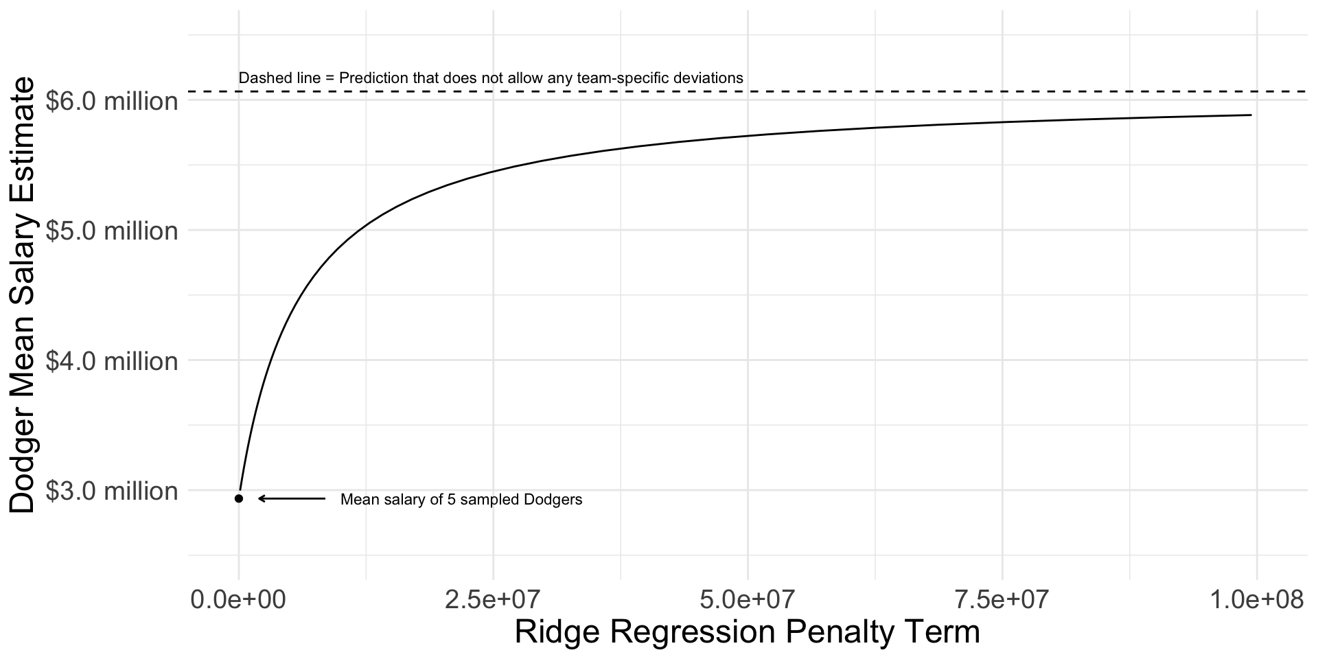

We will discuss how to choose the value of lambda more in two weeks when we discuss data-driven selection of an estimator.

Performance over repeated samples

The ridge regression estimator has intuitive performance across repeated samples: the variance of the estimates decreases as the value of the penalty parameter $\lambda$ rises. The biase of the estimates also increases as the value of $\lambda$ increases. The optimal value of $\lambda$ is a problem-specific question that requires one to balance the tradeoff between bias and variance.

Code

many_sample_estimates_ridge <- foreach(
  repetition = 1:100, .combine = "rbind"
) %do% {
  # Draw a sample from the population
  baseball_sample <- baseball_population |>
    group_by(team) |>
    slice_sample(n = 5) |>
    ungroup()
  # Apply the estimator to the sample# Learn a model in the sample
  ridge <- glmnet(
    x = model.matrix(~ -1 + team_past_record + team, data = baseball_sample),
    y = baseball_sample$salary,
    penalty.factor = c(0,rep(1,30)),
    alpha = 0
  )
  # Predict for our target population
  fitted <- predict(
    ridge, 
    s = ridge$lambda[c(20,60,80)],
    newx = model.matrix(~-1 + team_past_record + team, data = baseball_sample)
  )
  colnames(fitted) <- c("Large Lambda Value","Medium Lambda Value","Small Lambda Value")
  
  as_tibble(
    as.matrix(fitted[baseball_sample$team == "L.A. Dodgers",][1,]),
    rownames = "estimator"
  ) |>
    rename(estimate = V1)
}
# Visualize
many_sample_estimates_ridge |>
  mutate(estimator = fct_rev(estimator)) |>
  ggplot(aes(x = estimator, y = estimate)) +
  geom_jitter(width = .2, height = 0) +
  scale_y_continuous(
    name = "Dodger Mean Salary", 
    labels = label_currency(
      scale = 1e-6, accuracy = .1, suffix = " million"
    )
  ) +
  theme_minimal() +
  scale_x_discrete(
    name = "Estimator"
  ) +
  ggtitle(NULL, subtitle = "Each dot is an estimate in one sample from the population") +
  geom_hline(yintercept = true_dodger_mean, linetype = "dashed") +
  annotate(geom = "text", x = .4, y = true_dodger_mean, hjust = 0, vjust = .5, label = "Truth in\npopulation", size = 3)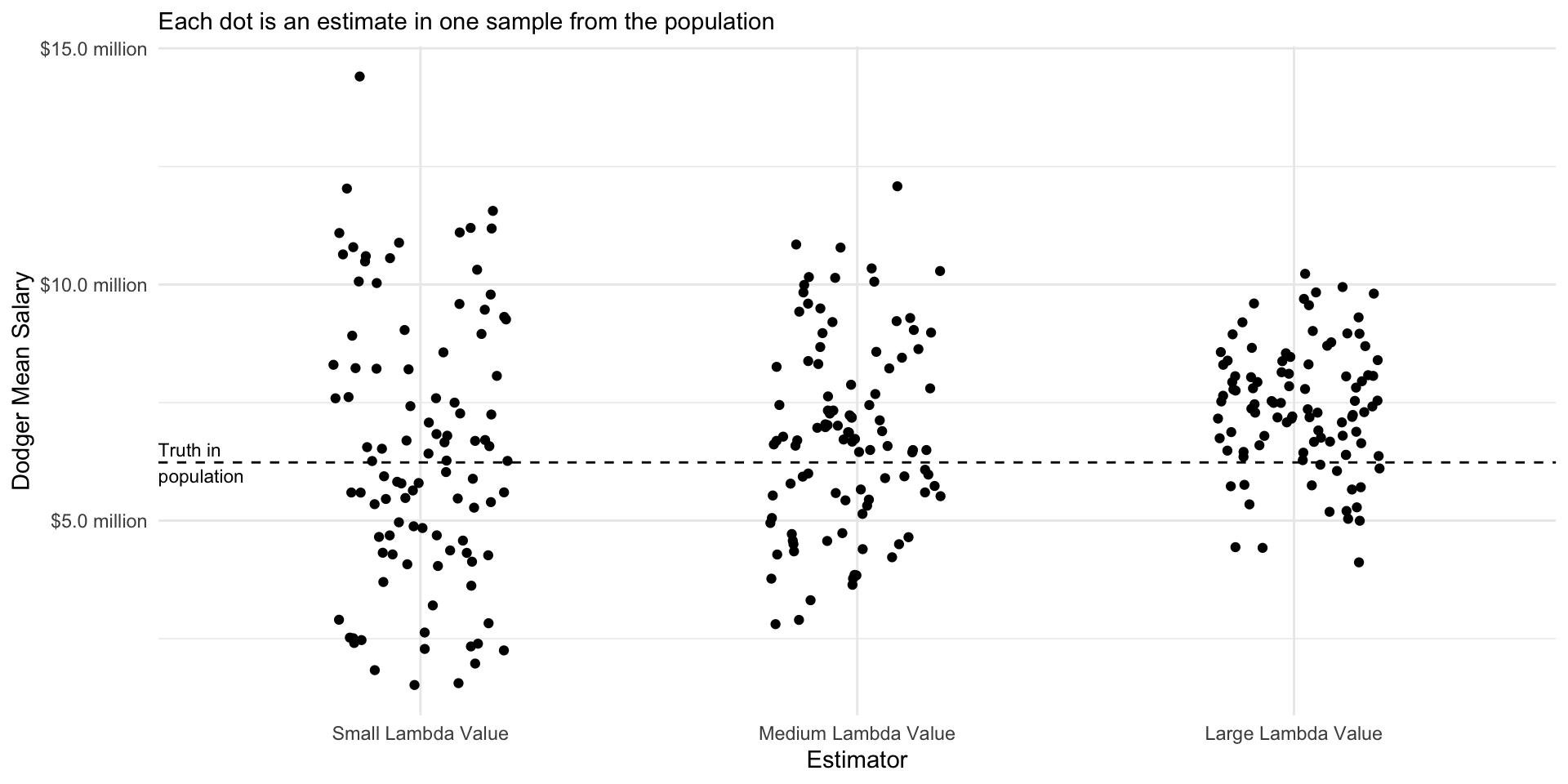

Connections: Multilevel model and ridge regression

multilevel <- lmer(salary ~ 1 + (1 | team), data = baseball_sample)

Code

yhat_multilevel <- baseball_sample |>
  mutate(yhat_multilevel = predict(multilevel)) |>
  distinct(team, yhat_multilevel)
lambda_equivalent <- as_tibble(VarCorr(multilevel)) |>
  select(grp, vcov) |>
  pivot_wider(names_from = "grp", values_from = "vcov") |>
  mutate(lambda_equivalent = Residual / team) |>
  pull(lambda_equivalent)

I will also fit ridge regression with $\lambda$ set to 9.

Code

X <- model.matrix(~ -1 + team, data = baseball_sample)
y_centered <- baseball_sample$salary - mean(baseball_sample$salary)
beta_ridge <- solve(
  t(X) %*% X + diag(rep(lambda_equivalent,ncol(X))), 
  t(X) %*% y_centered
)
yhat_ridge <- beta_ridge + mean(baseball_sample$salary)

Finally, we create a tibble with both the ridge regression and multilevel model estimates.

Code

both_estimators <- as_tibble(rownames_to_column(data.frame(yhat_ridge))) |>
  rename(team = rowname) |>
  mutate(team = str_remove(team,"team")) |>
  left_join(yhat_multilevel, by = join_by(team))

Connections: Multilevel model and ridge regression

Code

p <- both_estimators |>
  ggplot(aes(x = yhat_ridge, y = yhat_multilevel, label = team)) +
  geom_abline(intercept = 0, slope = 1) +
  scale_x_continuous(
    name = "Ridge Regression",
    labels = label_currency(
      scale = 1e-6, accuracy = .1, suffix = " million"
    )
  ) +
  scale_y_continuous(
    name = "Multilevel Model",,
    labels = label_currency(
      scale = 1e-6, accuracy = .1, suffix = " million"
    )
  ) +
  theme_minimal() +
  geom_point(alpha = 0) +
  theme(text = element_text(size = 18))
p

Connections: Multilevel model and ridge regression

Code

p + 
  geom_point()

Connections: Multilevel model and ridge regression

Multilevel model:

\[ \begin{aligned} Y_{ti} &\sim \text{Normal}(\mu_t,\sigma^2) \\ \mu_t &\sim \text{Normal}(\mu_0, \tau^2) \end{aligned} \] Estimates of $\mu_t$ given $\hat\mu_0$, $\hat\tau^2$, and $\hat\sigma^2$:

\[ \hat\mu_t^\text{Multilevel} = \frac{\sum_{i}Y_{ti} + \frac{\hat\sigma^2}{\hat\tau^2}\hat\mu_0}{n_t + \frac{\hat\sigma^2}{\hat\tau^2}} \]

Connections: Multilevel model and ridge regression

\[ \hat{\vec\mu}^\text{Ridge} = \underset{\vec\mu}{\text{arg min}} \underbrace{\sum_t\sum_i \left(Y_{it}-\mu_t\right)^2}_\text{Sum of Squared Error} + \underbrace{\lambda\sum_t \left(\mu_t - \hat\mu_0\right)^2}_\text{Penalty} \]

Rearranged to:

\[ \hat{\vec\mu}^\text{Ridge} = \underset{\vec\mu}{\text{arg min}} \sum_t\left(\sum_i \left(Y_{it}-\mu_t\right)^2 + \lambda\left(\hat\mu_0 - \mu_t\right)^2\right) \]

Connections: Multilevel model and ridge regression

\[ \hat{\vec\mu}^\text{Ridge} = \underset{\vec\mu}{\text{arg min}} \sum_t\left(\sum_i \left(Y_{it}-\mu_t\right)^2 + \lambda\left(\hat\mu_0 - \mu_t\right)^2\right) \]

Result:

\[ \hat\mu_t^\text{Ridge} = \frac{\sum_i Y_{it} + \lambda\hat\mu_0}{n_t + \lambda} \]

Connections: Multilevel model and ridge regression

Multilevel:

\[ \hat\mu_t^\text{Multilevel} = \frac{\sum_{i}Y_{ti} + \frac{\hat\sigma^2}{\hat\tau^2}\hat\mu_0}{n_t + \frac{\hat\sigma^2}{\hat\tau^2}} \]

Ridge:

\[ \hat\mu_t^\text{Ridge} = \frac{\sum_i Y_{it} + \lambda\hat\mu_0}{n_t + \lambda} \]

LASSO

LASSO regression

Outcome model similar to ridge:

\[ Y_{ti} = \alpha + \beta X_t + \gamma_{t} + \epsilon_{ti} \]

Loss function penalty has absolute value:

\[ \underbrace{\sum_t\sum_i\left(Y_{ti} - \left(\alpha + \beta X_t + \gamma_{t}\right)\right)^2}_\text{Sum of Squared Error} + \underbrace{\lambda\sum_t\lvert\gamma_t\rvert}_\text{Penalty} \]

LASSO: In code

library(glmnet)

lasso <- glmnet(
  x = model.matrix(~ -1 + team_past_record + team, data = baseball_sample),
  y = baseball_sample$salary,
  penalty.factor = c(0,rep(1,30)),
  # Choose LASSO (alpha = 1) instead of ridge (alpha = 0)
  alpha = 1
)

LASSO estimates

Code

p_lasso <- baseball_sample |>
  group_by(team) |>
  mutate(nonparametric = mean(salary)) |>
  ungroup() |>
  mutate(
    fitted = predict(
      lasso, 
      s = lasso$lambda[20],
      newx = model.matrix(~-1 + team_past_record + team, data = baseball_sample)
    )
  ) |>
  distinct(team, team_past_record, fitted, nonparametric) |>
  ungroup() |>
  ggplot(aes(x = team_past_record)) +
  geom_point(aes(y = nonparametric)) +
  geom_abline(
    intercept = coef(lasso, s = lasso$lambda[20])[1], 
    slope = coef(lasso, s = lasso$lambda[20])[2], 
    linetype = "dashed"
  ) +
  geom_segment(
    aes(y = nonparametric, yend = fitted),
    arrow = arrow(length = unit(.05,"in"))
  ) +
  geom_point(aes(y = nonparametric)) +
  #ggrepel::geom_text_repel(aes(y = fitted, label = team), size = 2) +
  theme_minimal() +
  theme(text = element_text(size = 18)) +
  scale_y_continuous(
    name = "Team Mean Salary in 2023", 
    labels = label_currency(
      scale = 1e-6, accuracy = .1, suffix = " million"
    )
  ) +
  scale_x_continuous(name = "Team Past Record: Proportion Wins in 2022") +
  ggtitle("LASSO regression on a sample of 5 players per team",
          subtitle = "Points are nonparametric sample mean estimates.\nArrow ends are ridge regression estimates.\nDashed line is the unregularized component of the model.")
p_lasso

LASSO estimates

Code

fitted <- predict(
  lasso, 
  newx = model.matrix(~-1 + team_past_record + team, data = baseball_sample)
)
dodgers_sample_mean <- baseball_sample |>
  filter(team == "L.A. Dodgers") |>
  summarize(salary = mean(salary)) |>
  pull(salary)
ols_estimate <- predict(
  lm(salary ~ team_past_record, data = baseball_sample),
  newdata = baseball_sample |> filter(team == "L.A. Dodgers") |> slice_head(n = 1)
)
tibble(estimate = fitted[baseball_sample$team == "L.A. Dodgers",][1,],
       lambda = lasso$lambda) |>
  ggplot(aes(x = lambda, y = estimate)) +
  geom_line() +
  scale_y_continuous(
    name = "Dodger Mean Salary Estimate", 
    labels = label_currency(
      scale = 1e-6, accuracy = .1, suffix = " million"
    ),
    expand = expansion(mult = .2)
  ) +
  scale_x_continuous(
    name = "LASSO Regression Penalty Term",
    limits = c(0,2.5e6)
  ) +
  annotate(
    geom = "point", x = 0, y = dodgers_sample_mean
  ) +
  annotate(geom = "segment", x = 2.5e5, xend = 1e5, y = dodgers_sample_mean,
           arrow = arrow(length = unit(.05,"in"))) +
  annotate(
    geom = "text", x = 3e5, y = dodgers_sample_mean,
    label = "Mean salary of 5 sampled Dodgers",
    hjust = 0, size = 3
  ) +
  geom_hline(yintercept = ols_estimate, linetype = "dashed") +
  annotate(
    geom = "text",
    x = 0, y = ols_estimate, 
    label = "Dashed line = Prediction that does not allow any team-specific deviations", 
    vjust = -.8, size = 3, hjust = 0
  ) +
  theme_minimal() +
  theme(text = element_text(size = 18))

LASSO: Performance

Code

many_sample_estimates_lasso <- foreach(
  repetition = 1:100, .combine = "rbind"
) %do% {
  # Draw a sample from the population
  baseball_sample <- baseball_population |>
    group_by(team) |>
    slice_sample(n = 5) |>
    ungroup()
  # Apply the estimator to the sample# Learn a model in the sample
  lasso <- glmnet(
    x = model.matrix(~ -1 + team_past_record + team, data = baseball_sample),
    y = baseball_sample$salary,
    penalty.factor = c(0,rep(1,30)),
    alpha = 1
  )
  # Predict for our target population
  fitted <- predict(
    lasso, 
    s = lasso$lambda[c(15,30,45)],
    newx = model.matrix(~-1 + team_past_record + team, data = baseball_sample)
  )
  colnames(fitted) <- c("Large Lambda Value","Medium Lambda Value","Small Lambda Value")
  
  as_tibble(
    as.matrix(fitted[baseball_sample$team == "L.A. Dodgers",][1,]),
    rownames = "estimator"
  ) |>
    rename(estimate = V1)
}
# Visualize
many_sample_estimates_lasso |>
  mutate(estimator = fct_rev(estimator)) |>
  ggplot(aes(x = estimator, y = estimate)) +
  geom_jitter(width = .2, height = 0) +
  scale_y_continuous(
    name = "Dodger Mean Salary", 
    labels = label_currency(
      scale = 1e-6, accuracy = .1, suffix = " million"
    )
  ) +
  theme_minimal() +
  theme(text = element_text(size = 18)) +
  scale_x_discrete(
    name = "Estimator"
  ) +
  ggtitle(NULL, subtitle = "Each dot is an estimate in one sample from the population") +
  geom_hline(yintercept = true_dodger_mean, linetype = "dashed") +
  annotate(geom = "text", x = .4, y = true_dodger_mean, hjust = 0, vjust = .5, label = "Truth in\npopulation", size = 3)

Recap + Project Connection

Recap

A recipe for prediction:

model in learning data
predict in target population
average

Recap

Performance (expected squared error) can suffer from two sources:

bias (model approximation error)
variance (too many parameters)

Regularization balances these two concerns

Recap

OLS: No regularization
Ridge regression: Penalizes sum of squared coefficients
LASSO regression: Penalizes sum of absolute coefficients

Multilevel models regularize group-specific estimates depending on the within-group precision, a special case of ridge regression.

Generalizations of our estimators

Ridge regression: Applies well to many settings with a large number of parameters, regardless of whether they are groups.

\[ \hat{\vec\beta}^\text{Ridge} = \underset{\vec\beta}{\text{arg min}} \underbrace{\sum_i \left(Y_i - \left(\alpha + \vec{X}'\vec\beta\right)\right)^2}_\text{Sum of Squared Error} + \underbrace{\lambda\sum_p \beta_p^2}_\text{Penalty} \]

Generalizations of our estimators

LASSO regression: Applies well to many settings with a large number of parameters, regardless of whether they are groups.

Generalizations of our estimators

Multilevel models can have group-specific slopes

\[ \begin{aligned} Y_{gi} &\sim \text{Normal}\left(\alpha_g + \beta_g X_{gi}, \sigma^2\right) \\ \alpha_g &\sim \text{Normal}\left(\eta_0, \tau^2\right) \\ \beta_g &\sim \text{Normal}\left(\lambda_0, \delta^2\right) \end{aligned} \]

Generalizations of our estimators

Multilevel models can have more than two levels

\[ \begin{aligned} Y_{ijk} &\sim \text{Normal}\left(\alpha_{ij}, \sigma^2\right) \\ \alpha_{ij} &\sim \text{Normal}\left(\beta_{i}, \tau^2\right) \\ \beta_{i} &\sim \text{Normal}\left(\lambda, \delta^2\right) \end{aligned} \]

Reading (optional)

Multilevel models

Gelman & Hill 2006 for worked examples
Murphy 2012 ch 5.6.2 for a succinct mathematical presentation

Reading (optional)

Ridge & LASSO: Hastie, Tibshirani, & Friedman 2017 Ch 3.4

Ridge regression

Efron & Hastie 2016 Ch 7.3 (all of ch 7 is useful)
Murphy 2012 ch 7.5 for a Bayes view with lots of math

LASSO regression

Efron & Hastie 2016 Ch 16

Connection to project

In your project, do you have a variable that creates

many groups with
few observations per group?

Where else do you have many parameters to estimate?

How could penalized regression apply in your project?

Problem Set 2

Due Monday 9pm: link

Algorithms for prediction

Problem Set 1: Discussion

Problem Set 1: Discussion

Problem Set 1: Discussion

Problem Set 1: Discussion

Goals for today

Data

Data: Baseball salaries

Data: Baseball salaries

Data: Baseball salaries

Data: Baseball salaries

Data: Baseball salaries

Task

Task: Predict Dodger mean salary

Task: Predict Dodger mean salary

Task: Predict Dodger mean salary

Task: Predict Dodger mean salary

Task: Predict Dodger mean salary

Task: Predict Dodger mean salary

Task: Predict Dodger mean salary

Task: Predict Dodger mean salary

Task: Create data to predict

OLS

Ordinary Least Squares: Model

Ordinary Least Squares: Predict

Ordinary Least Squares: Average

Performance of OLS

Performance of OLS: Estimator function

Performance of OLS: Estimator function

Performance of OLS: Estimator function

Performance of OLS: Estimator function

Approximation Error

Model approximation error

Model approximation error

OLS with many parameters

Regularization

Regularization

Regularization

Regularization: How much?

Regularization: How much?

Multilevel models

Multilevel models: Idea

Multilevel models: Code

Multilevel models: Intuition

Multilevel models: Intuition

Multilevel models: Performance

Multilevel models: In math

Ridge regression

Ridge regression

Ridge regression

Ridge regression: Code

Ridge regression: Estimates

Ridge regression: Penalty parameter \(\lambda\) controls shrinkage

Ridge regression: Penalty parameter \(\lambda\) controls shrinkage

Performance over repeated samples

Connections: Multilevel model and ridge regression

Connections: Multilevel model and ridge regression

Connections: Multilevel model and ridge regression

Connections: Multilevel model and ridge regression

Connections: Multilevel model and ridge regression

Connections: Multilevel model and ridge regression

Connections: Multilevel model and ridge regression

Connections: Multilevel model and ridge regression

LASSO

LASSO regression

LASSO: In code

LASSO estimates

LASSO estimates

LASSO estimates

LASSO: Performance

Recap + Project Connection

Recap

Recap

Recap

Generalizations of our estimators

Generalizations of our estimators

Generalizations of our estimators

Generalizations of our estimators

Reading (optional)

Reading (optional)