Evaluate Models

This page presents a $\hat{Y}$ view of what it means for one model to outperform another model. We first discuss in a simulated setting where we generate many samples from the population and directly observe performance of estimators across those simulated samples. Then, we discuss how one can evaluate performance in the more realistic setting in which only one sample from the population is available.

To run the code on this page, you will need the tidyverse package.

library(tidyverse)

We will also set the seed so that it is possible to exactly reproduce these results.

set.seed(90095)

Simulation: Many samples from the population

simulate a sample of 100 cases
apply each model
compare to the full-data estimate for the target subgroup

See the previous page for code to simulate a sample.

Estimator functions

The functions below is an estimator: it take data in and returns estimates. This function can be applied with the flat, linear, and quadratic models defiend on the previous page.

estimator <- function(
    data, # from simulate()
    model_name # one of "flat", "linear", "quadratic"
) {
  # Estimate a regression model
  if (model_name == "flat") {
    fit <- lm(log(income) ~ sex, data = data)
  } else if (model_name == "linear") {
    fit <- lm(log(income) ~ sex * age, data = data)
  } else if (model_name == "quadratic") {
    fit <- lm(log(income) ~ sex * poly(age,2), data = data)
  }
  # Define x-values at which to make predictions
  to_predict <- tibble(
    sex = c("female","male"),
    age = c(30,30)
  )
  # Make predictions
  predicted <- to_predict |>
    mutate(estimate = predict(fit, newdata = to_predict)) |>
    # Transform from log scale to dollars scale
    mutate(estimate = exp(estimate)) |>
    # Append information for summarizing later
    mutate(
      model_name = model_name,
      sample_size = nrow(data)
    )
  # Return the predicted estimates
  return(predicted)
}

As an illustration, here is the linear estimator applied to a simulated sample

simulated <- simulate(n = 100)

estimator(data = simulated, model_name = "linear")

# A tibble: 2 × 5
  sex      age estimate model_name sample_size
  <chr>  <dbl>    <dbl> <chr>            <int>
1 female    30   38436. linear             100
2 male      30   51877. linear             100

Apply estimators in repeated samples

How do our estimators perform in repeated samples? In actual problems, one only has one sample. But we created this exercise so that we can use simulate() to simulate many samples from a known data generating process. The code below applies the estimator to many samples of size 100.

We first prepare for parallel computing.

library(foreach)
library(doParallel)
library(doRNG)
cl <- makeCluster(detectCores())
registerDoParallel(cl)

Then we apply the estimator many times at each of a series of sample sizes.

simulations <- foreach(
  repetition = 1:1000, 
  .combine = "rbind", 
  .packages = "tidyverse"
) %dorng% {
  foreach(n_value = c(50,100,200,500,1000), .combine = "rbind") %do% {
    # Simulate data
    simulated <- simulate(n = n_value)
    # Apply the three estimators
    flat <- estimator(data = simulated, model_name = "flat")
    linear <- estimator(data = simulated, model_name = "linear")
    quadratic <- estimator(data = simulated, model_name = "quadratic")
    # Return estimates
    all_estimates <- rbind(flat, linear, quadratic)
    return(all_estimates)
  }
}

Visualize estimator performance

For simplicity, we first focus on one estimand and sample size: modeling the geometric mean of 30-year-old female incomes with a sample size of $n = 100$. Despite having good performance in the population, the quadratic model has poor performance at this sample size because it has high variance!

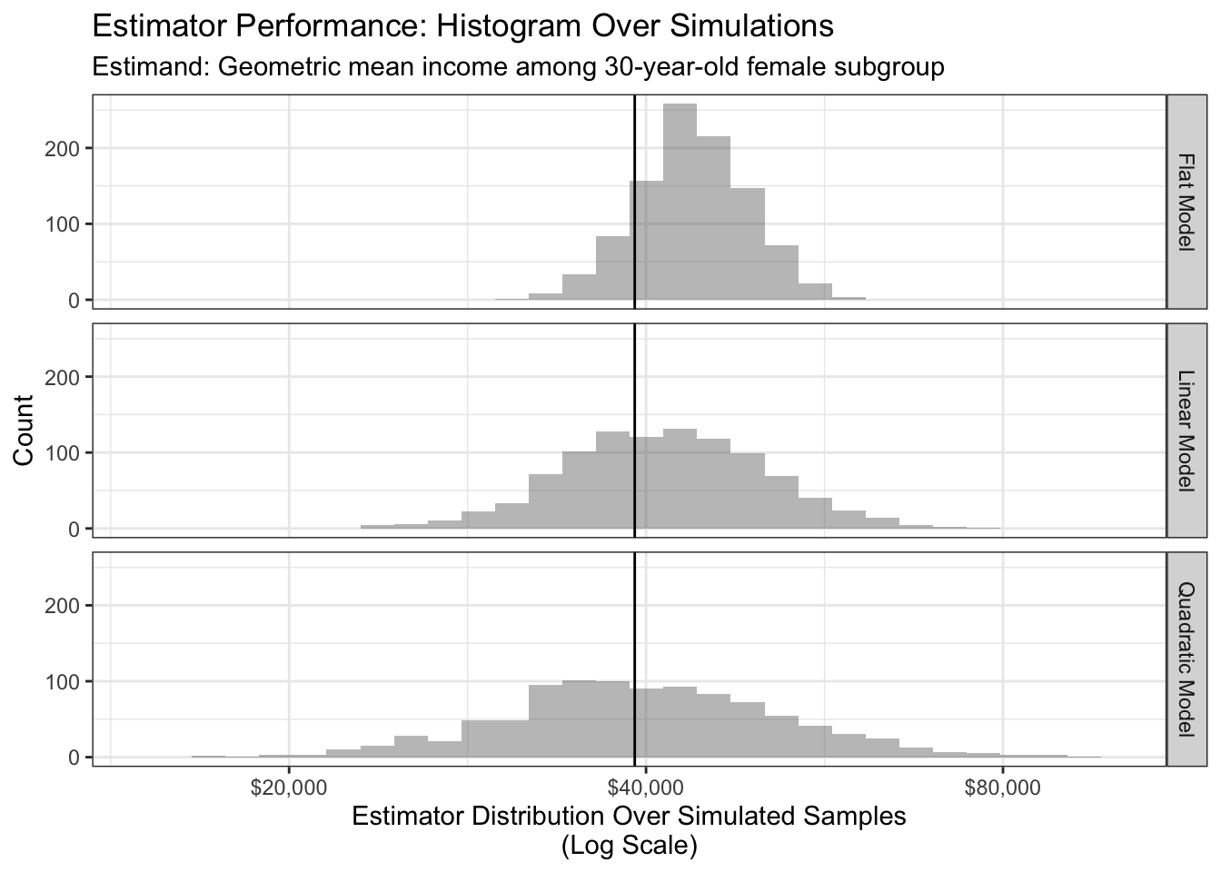
To aggregate simulations to a summary score, we use mean squared error (MSE) on the scale of log incomes.

\[\begin{aligned} \theta(\vec{x}) &= \text{True geometric mean in subgroup }\vec{x} \\ \hat\theta_r(\vec{x}) &= \text{Estimated geometric mean in subgroup }\vec{x}\text{ in simulated sample }r \\ \widehat{\text{MSE}}\bigg(\hat\theta(\vec{x})\bigg) &= \frac{1}{R}\sum_{r=1}^R \left(\text{log}(\hat\theta) - \text{log}(\theta)\right)^2 \end{aligned}\]

To calculate the MSE, we need the true values from our simulation. The code below is somewhat opaque because it requires you to know something about how we generated the data. In this code, meanlog is the mean log income in each sex $\times$ age $\times$ year subgroup, estimated in the full ACS. The weight corresponds to the size of the subgroup; later years have greater weight because the total population was greater then, for example. We aggregate to truth within sex $\times$ age subgroups.

truth <- read_csv("https://ilundberg.github.io/description/assets/truth.csv") |>
  group_by(sex, age) |>
  summarize(
    truth = exp(weighted.mean(meanlog, w = weight)),
    .groups = "drop"
  )

The code below merges the truth with the simulated estimates and calculates aggregate performance metrics: bias, variance, and mean squared error.

aggregate_performance <- simulations |>
  # Merge in the true values from the simulation
  left_join(truth, by = join_by(sex, age)) |>
  # Convert to log scale
  mutate(
    estimate = log(estimate), 
    truth = log(truth)
  ) |>
  # Calculate aggregate performance within
  # population subgroups (sex, age)
  # and simulation settings (model_name, sample_size)
  group_by(sex, age, model_name, sample_size) |>
  summarize(
    bias = mean(estimate - truth),
    variance = var(estimate),
    mse = mean((estimate - truth) ^ 2),
    .groups = "drop"
  )

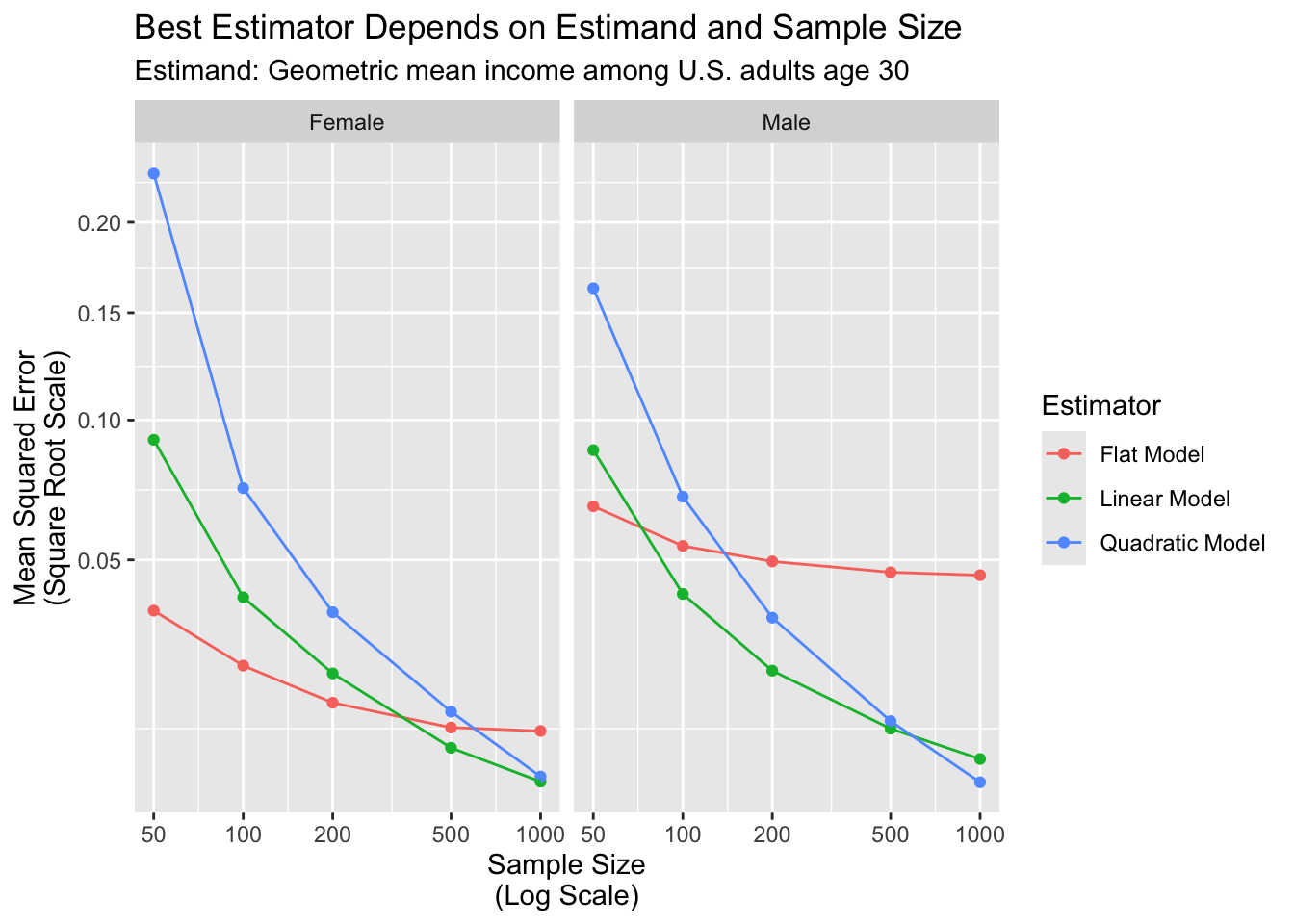
The graph below visualizes aggregate performance measured by mean squared error.

Conclusions: Many-samples simulation

The results show how the more complex models perform better than simpler models only at larger sample sizes.

For the male subgroup,

a flat model is best at $n = 50$
a linear model becomes best at $n = 100$
a quadratic model becomes best at $n ={}$1,000

For the female subgroup,

a flat model is best at $n = 50, 100, 200$
a linear model becomes best at $n = 500$
a quadratic model may become best at an untested sample size greater than $n ={}$1,000

There are two main conclusions from this illustration. Which estimator is best is a question that

depends on the estimand (male or female subgroup), and
depends on the sample size

Further, although the quadratic fit is best in the population (previous page), a very large sample size is needed before it is best in a sample. This is a reminder that more complex models do not necessarily outperform simpler models, especially in small samples.

Realistic: One sample from the population

In the real world, we cannot evaluate performance over many samples from the population. We typically have only one sample! This section is about evaluating performance when only one sample is available.

The code below generates one sample.

simulated <- simulate(n = 100) |>
  # To track the units in this sample, we will add an id column
  mutate(id = 1:n())

One way to evaluate in one sample is to use a split-sample procedure:

Split into learning and evaluation sets
Estimate models in the learning set
Evaluate in the evaluation set

The advantage of this procedure is that a complex model that performs well in the learning set may not generalize well to the evaluation set. Through sample splitting, we can select a model that performs well at roughly our actual sample size (at least, at 50% of our sample size).

Split into learning and evaluation sets

Create a learning set with half of the cases.

learning <- simulated |>
  slice_sample(prop = .5)

Create an evaluation set with the other half.

evaluation <- simulated |>
  anti_join(learning, by = join_by(id))

Estimate models in the learning set

Next, estimate the models in the learning set.

flat <- lm(log(income) ~ sex, data = learning)
linear <- lm(log(income) ~ sex * age, data = learning)
quadratic <- lm(log(income) ~ sex * poly(age,2), data = learning)

Evaluate in the evaluation set

Use them to predict in the evaluation set.

predicted <- evaluation |>
  mutate(
    flat = predict(flat, newdata = evaluation),
    linear = predict(linear, newdata = evaluation),
    quadratic = predict(quadratic, newdata = evaluation)
  )

Aggregate prediction errors in the evaluation set to produce mean squared error estimates for each model.

performance <- predicted |>
  # Select the actual and predicted values
  mutate(actual = log(income)) |>
  select(actual, flat, linear, quadratic) |>
  # Make a long dataset for ease of analysis
  pivot_longer(cols = -actual, names_to = "model_name", values_to = "prediction") |>
  # Create a column with errors
  mutate(squared_error = (actual - prediction) ^ 2) |>
  # Summarize mean squared error
  group_by(model_name) |>
  summarize(mse = mean(squared_error)) |>
  print()

# A tibble: 3 × 2
  model_name   mse
  <chr>      <dbl>
1 flat       0.635
2 linear     0.632
3 quadratic  0.711

Our split-sample procedure estimates that the linear model has the best performance!

Difficulties in split-sample model evaluation

the estimated performance may itself be statistically uncertain
if the best model in one subgroup is different from the best in another subgroup, then a sample-average MSE may not be optimal for selecting for our task