library(tidyverse)
data <- read_csv("https://ilundberg.github.io/causalestimators/data/data.csv")Data
This page uses two main datasets: one very simple simulated data, and one more realistic simulation.
Simple simulation
The simple simulation data are available in data.csv.
This simple simulation contains \(n = 500\) observations. Each observation contains several observed variables:
L1A numeric confounderL2A numeric confounderAA binary treatmentYA numeric outcome
Each observation also contains outcomes that we know only because the data are simulated. These variables are useful as ground truth in simulations.
propensity_scoreThe true propensity score \(P(A = 1 \mid \vec{L})\)Y0The potential outcome under controlY1The potential outcome under treatment
Click here to see the code that simulated the data
If you want to generate your own simulated sample, below is the code we used.
Below is code you can use to generate your own simulated sample, if you wish.
library(dplyr)If you want your simulation to match our numbers exactly, add a line to set your seed.
set.seed(90095)n <- 500
data <- tibble(
L1 = rnorm(n),
L2 = rnorm(n)
) |>
# Generate potential outcomes as functions of L
mutate(Y0 = rnorm(n(), mean = L1 + L2, sd = 1),
Y1 = rnorm(n(), mean = Y0 + 1, sd = 1)) |>
# Generate treatment as a function of L
mutate(propensity_score = plogis(-2 + L1 + L2)) |>
mutate(A = rbinom(n(), 1, propensity_score)) |>
# Generate factual outcome
mutate(Y = case_when(A == 0 ~ Y0,
A == 1 ~ Y1))A simulation is nice because the answer is known. In this simulation, the conditional average causal effect of A on Y equals 1 at any value of L1 and L_2.
Realistic simulation
The more realistic simulation is based on an ongoing project with Soonhong Cho, in which we use NLSY97 data to estimate the causal effect of motherhood on employment and wages. You can load a simulated version of these data with the code below.
library(tidyverse)
motherhood_simulated <- read_csv("https://ilundberg.github.io/causalestimators/data/motherhood_simulated.csv")
The simulated data
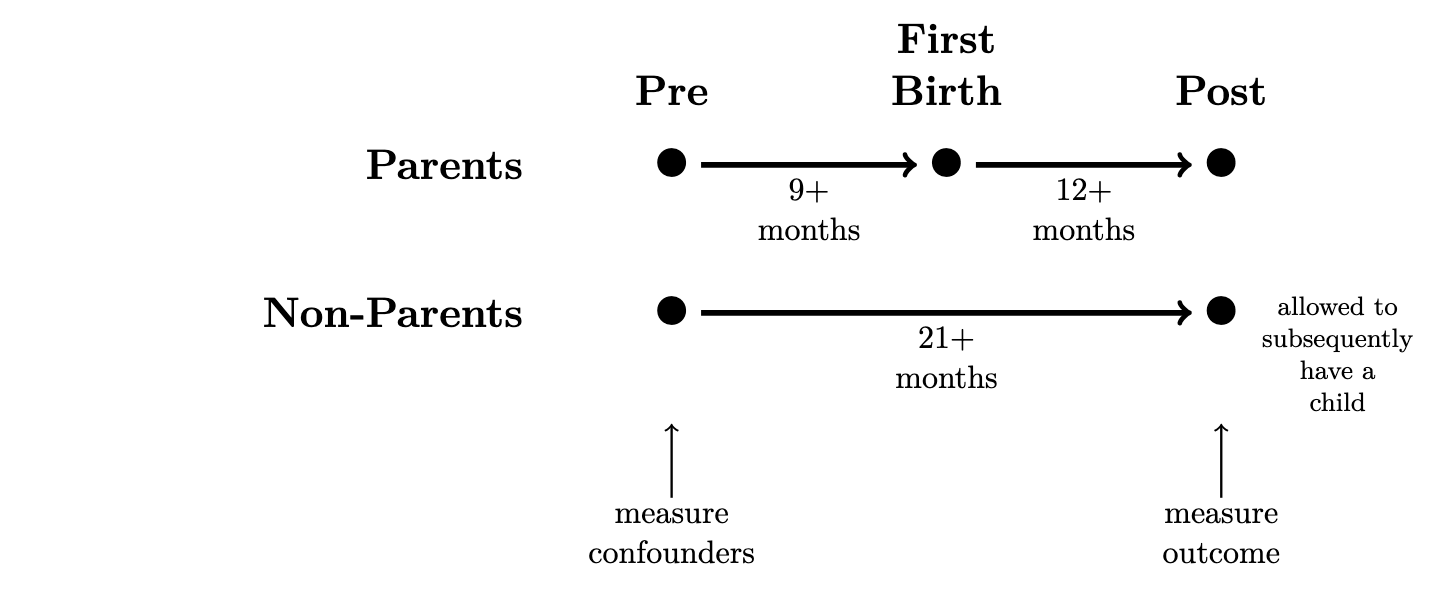
This problem set estimates the causal effect of motherhood on mothers’ employment, using data simulated to approximate data that exist in the National Longitudinal Survey of Youth 1997 cohort. The NLSY97 interviews people repeatedly across years. We manipulated these data so that each row contains information from a pre- and a post-observation, separated by 21+ months. In the pre-observation, we measure confounding variables. In the post-observation, we measure the outcome (y, employment). Between the pre- and post-observation, some women experience a first birth (treated == TRUE) and others do not (treated == FALSE).
The dataset motherhood_simulated.csv contains the following variables.
observation_idis an index for each observationsampling_weightis the weight due to unequal probability samplingtreatedindicates a first birth (TRUEorFALSE)- This occurred between the pre- and post-periods.
yis the outcome, codedTRUEif employed orFALSEif not employed.- This was measured in the post-period.
The data include a set of variables measured in the pre-period. We will consider these to be a sufficient adjustment set. These were measured in the pre-period.
raceis a categorical variable codedHispanic,Non-Hispanic Black, andNon-Hispanic Non-Blackpre_ageis age in yearspre_educis an ordinal variable for educational attainment, codedLess than high school,High school,2-year degree, and4-year degreewith those with higher levels of education also coded in this last categorypre_maritalis a categorical variable of marital status, codedno_partner,cohabiting, ormarriedpre_employedis a lag measure of employment in the prior survey wave, codedTRUEandFALSEpre_fulltimeindicates full-time employment in the prior survey wave, codedTRUEandFALSEpre_tenureis years of experience with a current employer, as of the prior survey wavepre_experienceis total years of full-time work experience, as of the prior survey wave