Building Intuition

Before diving into a more complex simulated setting, this page builds intuition for causal estimators in a simple setting with only 6 observations. At confounder value 1, 2 out of 3 are treated. At confounder value 2, 1 out of 3 is treated.

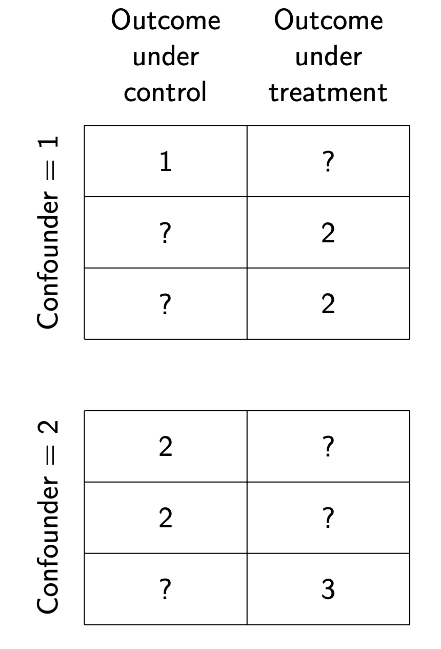
We assume causal identification given the confounder. The causal problem is to use the observed data to learn about the missing values.

Outcome modeling

One strategy is to estimate an outcome model for the conditional mean of the observed outcomes.

\[E(Y\mid A, X) = \alpha + \beta X + \gamma A\]

In these data, we would estimate \(\hat\alpha = 0\), \(\hat\beta = 1\), and \(\hat\gamma = 1\). We could then predict the counterfactual outcomes.

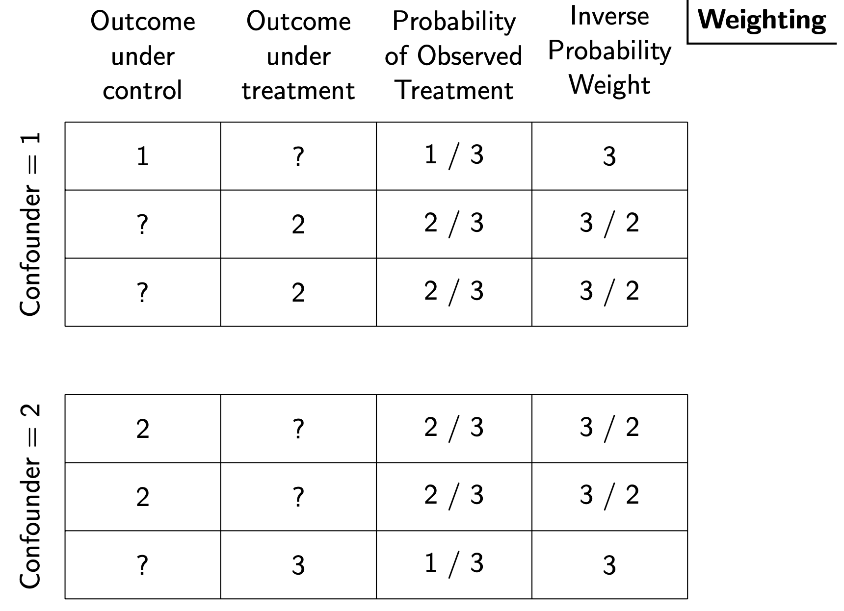
Inverse probability weighting

Another strategy is to consider the treated units as a sample of all units, drawn with unequal probabilities across confounder values. Likewise, for the control units. Just as in sampling we would weight by the inverse probability of sample inclusion, we can weight by the inverse probability of the observed treatment.

Matching

A third is to find for each unit a matched case that had the other treatment condition. We then impute the missing outcome value by the observed outcome of the matched case.

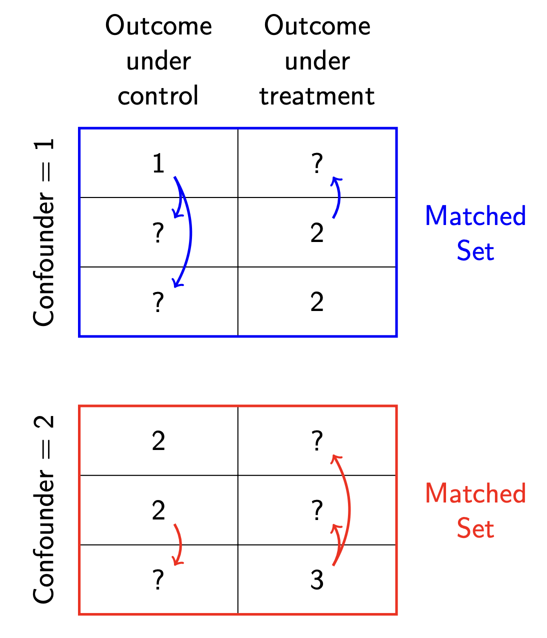
Matching can be conceptualized as a special case of outcome modeling, where the outcome model is a nearest neighbor estimator.

What to do next

Now that you have a conceptual idea of these strategies, move on to the next pages to practice them with simulated data.