2 Concepts in detail

This section provides a more detailed overview of the use of gapclosing().

It is structured from the perspective of the three key tasks for the researcher:

define the intervention
make causal assumptions for identification
specify a treatment and/or outcome model

Along the way, this section introduces many of the possible arguments in a gapclosing() call.

2.1 Define the intervention

To answer a gap-closing question, we first need to define what that intervention would be. To what treatment value would units be counterfactually assigned? There are several options.

Option 1. Set counterfactual_assignments = 0 or counterfactual_assignments = 1. In this case, we are studying the disparity we would expect if a random person of each category were assigned control or if assigned treatment (respectively).
Option 2. Set counterfactual_assignments = \(\pi\) for some \(\pi\) between 0 and 1. In this case, we are studying the disparity we would expect if a random person of each category were assigned to treatment with probability \(\pi\) and to control with probability \(1 - \pi\).
Option 3. Assign treatments by a probability \(\pi_i\) that may differ for each person \(i\). In this case, we create a vector \(\vec\pi\) of length \(n\) and pass that in the counterfactual_assignments argument.

Example. We are interested in the disparity across populations defined by category that would persist under counterfactual assignment to set treatment to the value 1. counterfactual_assignments = 1

2.2 Make causal assumptions for identification

The package does help you with this step. Gap-closing estimands involve unobserved potential outcomes. Because they are unobserved, the data cannot tell us which variables are needed for estimation. Instead, that is a conceptual choice to be carried out with tools like Directed Acyclic Graphs (DAGs). See the accompanying Lundberg (2022) paper for more on identification.

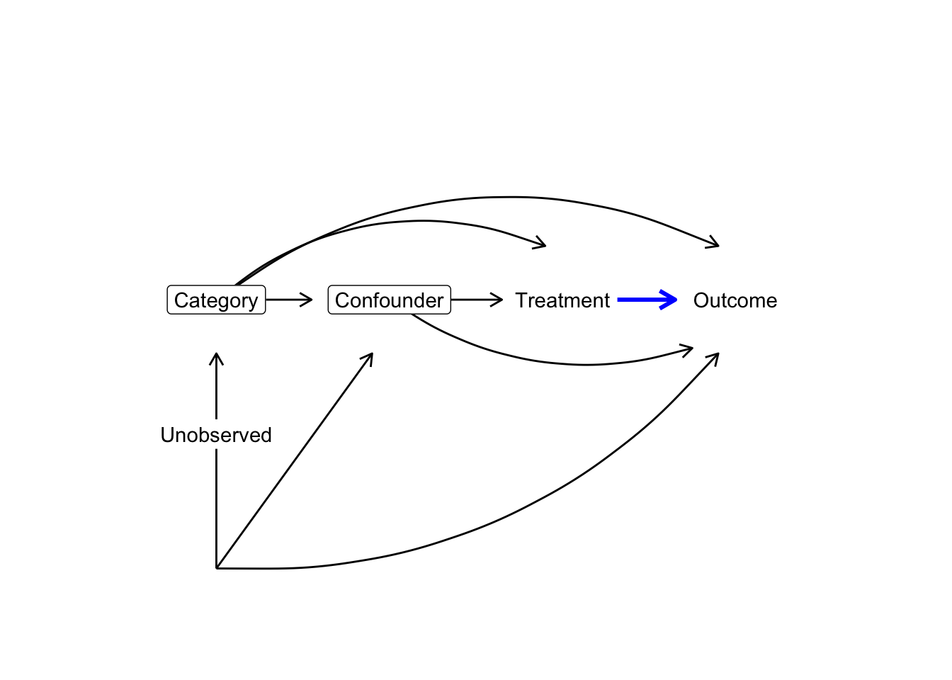
Example. Assume that the set of variables \(\{X,L\}\) is a sufficient conditioning set to identify the gap-closing estimand. Formally, this requires us to assume that within each stratum of \(X\) and \(L\) the expected value of the potential outcome \(Y(1)\) is the same as the expected value among units who factually have \(T = 1\) within those strata. \[\mathbb{E}(Y(1)\mid X, L) = \mathbb{E}(Y\mid X, L, T = 1)\] DAGs are a good way to reason about this assumption: in this example, conditioning (depicted by boxes) on category and confounder is sufficient to identify the causal effect of treatment (blue edge in the DAG), because doing so blocks all backdoor paths between the treatment and the outcome. Notably, the gap-closing estimand makes no claims about the causal effect of category since the counterfactual is defined over treatment only.

Once we select a sufficient conditioning set, those predictors will appear in both the treatment and/or the outcome model used for estimation.

2.3 Specify a treatment model and/or an outcome model

We need to estimate one or both of (1) the probability of treatment given confounders and (2) the conditional mean of the outcome given treatment and confounders. We do that by providing one or both of the following.

Provide a treatment_formula with the binary treatment variable on the left side and all confounders on the right side. This formula will be used in treatment_algorithm (see next step) to estimate the probability of treatment given confounders for each unit. Then, the sample-average outcome under counterfactual assignment to any given treatment can be estimated through inverse probability weighting among units who factually received that treatment.

Example.
treatment_formula = formula(outcome ~ confounder + category)

Provide an outcome_formula with the outcome variable on the left side and the treatment and all confounders on the right side. This formula will be used in outcome_algorithm (see next step) to estimate the conditional mean of the outcome given treatment and confounders. Then, it can be used to predict the potential outcome each unit would expect under any treatment of interest, given confounding variables.

Example.
outcome_formula = formula(outcome ~ confounder + category*treatment)

Whether treatment_formula or outcome_formula is left NULL will determine the estimation procedure.

If only treatment_formula is provided, then estimation will be by inverse probability of treatment weighting.
If only outcome_formula is provided, then estimation will be by prediction of unobserved potential outcomes (the \(g\)-formula, see Hernán and Robins (2021)).
If both treatment_formula and outcome_formula are provided, then the primary estimate will be doubly robust, with separate treatment and outcome modeling estimates accessible through the returned object.

2.3.1 Choose an estimation algorithm

The treatment_formula and outcome_formula are handed to treatment_algorithm and outcome_algorithm, which can take the following values.

glm (for treatment_algorithm only): A logistic regression model estimated by the glm function. If there are important interactions among treatment, category, and covariates, these should be included explicitly.
lm (for outcome_algorithm only): An OLS regression model estimated by the lm function. If there are important interactions among treatment, category, and covariates, these should be included explicitly.
ridge: A ridge (i.e. L₂-penalized) logistic regression model (for treatment_algorithm) or linear regression model (for outcome_algorithm) estimated by the glmnet function in the glmnet package (Friedman, Hastie, and Tibshirani 2010), with alpha = 0 to indicate the ridge penalty. Elastic net and lasso regression are not supported because those approaches could regularize some coefficients to exactly zero, and if you have chosen the needed confounders (step 2) then you would not want their coefficients to be regularized to zero. The penalty term is chosen by cv.glmnet and is set to the value lambda.min (see glmnet documentation). If there are important interactions among treatment, category, and covariates, these should be included explicitly.
gam: A Generalized Additive Model (logistic if used as treatment_algorithm, linear if used as outcome_algorithm) estimated by the gam function in the mgcv package (Wood 2017). The model formula should be specified as in the mgcv documentation and may include smooth terms s() for continuous covariates. If there are important interactions among treatment, category, and covariates, these should be included explicitly.
ranger: A random forest estimated by the ranger function in the ranger package (Wright and Ziegler 2017). If used as treatment_algorithm, one forest will be fit and predicted treatment probabilities will be truncated to the [.001,.999] range to avoid extreme inverse probability of treatment weights. If used as outcome_algorithm, the forest will be estimated separately on treated and control units; the treatment variable does not need to be included in outcome_formula in this case.

Example.
treatment_algorithm = "glm"
outcome_algorithm = "lm"

If the data are a sample from a population selected with unequal probabilities, you can also use the weight_name option to pass estimation functions the name of the sampling weight (a variable in data proportional to the inverse probability of sample inclusion). If omitted, a simple random sample is assumed.

2.3.2 Why doubly robust? A side note

Doubly-robust estimation yields advantages that can be conceptualized in two ways.

From the perspective of parametric models, if either the treatment or the outcome model is correct, then the estimator is consistent (Bang and Robins 2005). See Glynn and Quinn (2010) for an accessible introduction.
From the perspective of machine learning, double robustness adjusts for the fact that outcome modeling alone is optimized for the wrong prediction task. An outcome model would be optimized to predict where we observed data, but our actual task is to predict over a predictor distribution different from that which was observed (because the treatment has been changed). This is an opportunity to improve the predictions. By building a model of treatment, we can reweight the residuals of the outcome model to estimate the average prediction error over the space where we want to make predictions. Subtracting off this bias can improve the outcome modeling estimator. This pivot is at the core of moves toward targeted learning (Van der Laan and Rose 2011) and double machine learning (Chernozhukov et al. 2018), building on a long line of research in efficient estimation (Robins and Rotnitzky 1995; Hahn 1998).

Although double robustness has strong mathematical properties, in any given application with a finite sample it is possible that treatment or outcome modeling could outperform doubly-robust estimation. Therefore, the package supports all three approaches.

2.3.3 Why sample splitting? Another side note

Taking the bias-correction view of double robustness above, it is clear that sample splitting affords a further opportunity for improvement: if you learn an outcome model and estimate its average bias on the same sample, you might get a poor estimate of the bias. For this reason, one should consider using one sample (which I call data_learn) to learn the prediction functions and another sample (which I call data_estimate) to estimate the bias and aggregate to an estimate of the estimand.

In particular, the option sample_split = "cross_fit" allows the user to specify that estimation should proceed by a cross-fitting procedure which is analogous to cross-validation.

Split the sample into folds \(f = 1,\dots,\)n_folds (default here is n_folds = 2)
Use all folds except \(f'\) to estimate the treatment and outcome models
Aggregate to an estimate using the predictions in \(f'\)
Average the estimate that results from (2) and (3) repeated n_folds times with each fold playing the role of \(f'\) in turn

This is the procedure that Chernozhukov et al. (2018) argue is critical to double machine learning for causal estimation, although this type of sample splitting is not new (Bickel 1982).

If sample_split = "cross_fit", the default is to conduct 2-fold cross-fitting, but this can be changed with the n_folds argument. The user can also specify their own vector folds of fold assignments of length nrow(data), if there is something about the particular setting that would make a manual fold assignment preferable.

Example. (this is the default and can be left implicit)
sample_split = "one_sample"

2.3.4 Produce standard errors

The package supports bootstrapped standard error estimation. The procedure with bootstrap_method = "simple" (the default) is valid when the data are a simple random sample from the target population. In this case, each bootstrap iteration conducts estimation on a resampled dataset selected with replacement with equal probabilities. The standard error is calculated as the standard deviation of the estimate across bootstrap samples, and confidence intervals are calculated by a normal approximation.

Example. (line 2 is the default and can be left implicit)
se = T bootstrap_samples = 1000

In some settings, the sample size may be small and categories or treatments of interest may be rare. In these cases, it is possible for one or more simple bootstrap samples to contain zero cases in some (treatment \(\times\) category) cell of interest. To avoid this problem, bootstrap_method = "stratified" conducts bootstrap resampling within blocks defined by (treatment \(\times\) category). This procedure is valid if you assume that the data are selected at random from the population within these strata, so that across repeated samples from the true population the proportion in each stratum would remain the same.

Many samples are not simple random samples. In complex sample settings, users should implement their own standard error procedures to accurately capture sampling variation related to how their data were collected. The way the data were collected could motivate a resampling strategy to mimic the sources of variation in that sampling process, which the user can implement manually by calling gapclosing to calculate a point estimate on each resampled dataset with se = FALSE.

1 Big idea

3 Machine learning examples