1 Big idea

This part introduces the big ideas: why we should do this, what data look like, and what’s going on under the hood. It closes with basic package functionality.

1.1 Motivation

Gaps across social categories like race, class, and gender are important to understand. We would like to know whether there is anything we can do to close these gaps. What if we intervened to reduce incarceration or increase access to education? Would those interventions close gaps across categories of race, class, or gender?

These types of questions are at the core of a growing literature in epidemiology addresses these questions with techniques for causal decomposition analysis (VanderWeele and Robinson (2014), Jackson and VanderWeele (2018), Jackson (2020)). This package provides software to support inquiry into gap-closing estimands, as discussed in Lundberg (2022).

A guiding principle is to distinguish human tasks from software tasks that can be automated.

As a human, you will:

define the intervention
make causal assumptions for identification
specify a treatment model and/or an outcome model

Then package will:

estimate models
produce doubly-robust estimates
sample split to improve convergence
estimate standard errors by bootstrapping
visualize the result

1.2 Data structure

In a data frame data, we have a gap-defining category such as race, gender, or class. We have a binary treatment variable that could have counterfactually been different for any individual. We want to know the degree to which an intervention to change the treatment would close gaps across the categories.

These boxes will present an example.

Example. Suppose we have the following data.

\(X\) (category): Category of interest, taking values {A, B, C}

\(T\) (treatment): Binary treatment variable, taking values 0 and 1

\(L\) (confounder): A continuous confounding variable, Uniform(-1,1)

\(Y\) (outcome): A continuous outcome variable, conditionally normal

set.seed(08544)
library(gapclosing)
library(dplyr)
library(ggplot2)

simulated_data <- generate_simulated_data(n = 1000)
head(simulated_data)
#>   category confounder treatment    outcome
#> 1        C   1.640509         1 -0.7970377
#> 2        B   1.032373         0  1.9304909
#> 3        C   2.217630         1 -0.2009803
#> 4        A  -1.642914         0 -0.5015702
#> 5        A  -1.844897         0 -1.2027025
#> 6        A  -2.415100         0 -3.9288188

1.3 Coding from scratch

With the most simple models, you can carry out a gap-closing analysis without the software package. First, fit any prediction function for the outcome as a function of the category of interest, confounders, and treatment.

example_ols <- lm(outcome ~ category*treatment + confounder,
                  data = simulated_data)

For everyone in the sample, predict under a counterfactual treatment value (e.g., treatment = 1).

fitted <- simulated_data %>%
  mutate(outcome_under_treatment_1 = predict(example_ols,
                                             newdata = simulated_data %>%
                                               mutate(treatment = 1)))

Average the counterfactual estimates within each category.

fitted %>%
  # Group by the category of interest
  group_by(category) %>%
  # Take the average prediction
  summarize(factual = mean(outcome),
            counterfactual = mean(outcome_under_treatment_1))
#> # A tibble: 3 × 3
#>   category factual counterfactual
#>   <chr>      <dbl>          <dbl>
#> 1 A        -1.09           0.0488
#> 2 B        -0.0384        -0.0370
#> 3 C         0.495          0.132

The software package supports these steps as well as more complex things you might want:

three estimation strategies
- outcome prediction
- treatment prediction
- doubly robust estimation
machine learning prediction functions
counterfactual treatments that differ across units
bootstrapping for standard errors
easy visualization

1.4 Basic package functionality

The gapclosing() function estimates gaps across categories and the degree to which they would close under the specified counterfactual_assignments of the treatment.

estimate <- gapclosing(
  data = simulated_data,
  counterfactual_assignments = 1,
  outcome_formula = formula(outcome ~ confounder + category*treatment),
  treatment_formula = formula(treatment ~ confounder + category),
  category_name = "category",
  se = TRUE,
  # Setting bootstrap_samples very low to speed this tutorial
  # Should be set higher in practice
  bootstrap_samples = 20,
  # You can process the bootstrap in parallel with as many cores as available
  parallel_cores = 1
)

By default, this function will do the following:

Fit logistic regression to predict treatment assignment
Fit OLS regression to predict outcomes
Combine the two in a doubly-robust estimator estimated on a single sample
Return a gapclosing object which supports summary, print, and plot functions.

In this example, the plot(estimate) function produces the following visualization. The factual outcomes are unequal across categories, but the counterfactual outcomes are roughly equal. In this simulated setting, the intervention almost entirely closes the gaps across the categories.

plot(estimate)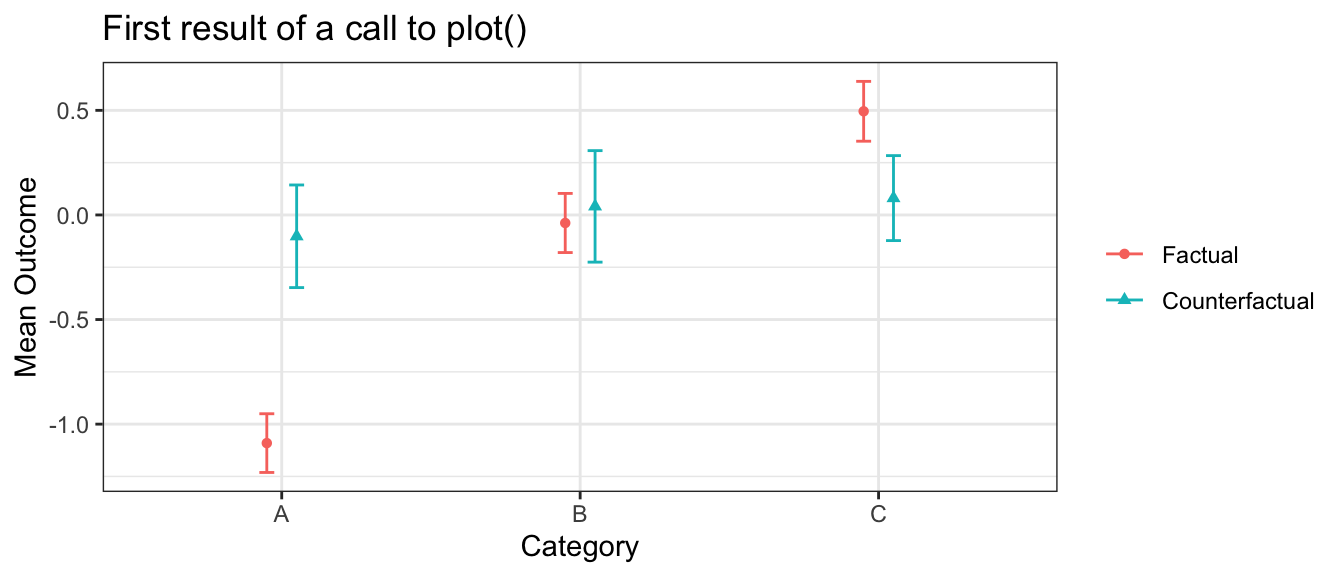

The disparityplot() function lets us zoom in on the factual and counterfactual disparity between two categories, of interest. In this case, we see that the intervention lifts outcomes in category A to be more comparable to category B. A disparityplot is a ggplot2 object and can be customized by passing additional layers.

disparityplot(estimate, category_A = "A", category_B = "B") +
  ggtitle("A disparityplot()")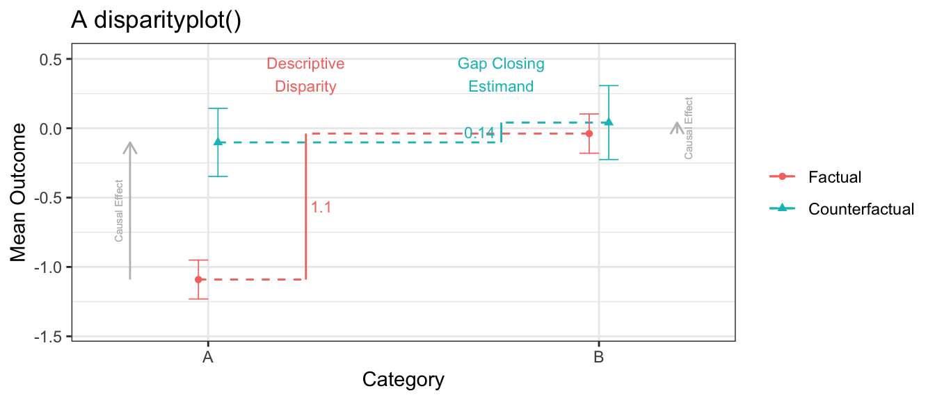

The summary function will print estimates, standard errors, and confidence intervals for all of these results.

summary(estimate)
#> Gap-closing estimates using doubly_robust estimation on one sample.
#> 
#> Treatment model was glm estimation with model formula:
#> formula(treatment ~ confounder + category)
#> 
#> Outcome model was lm estimation with model formula:
#> formula(outcome ~ confounder + category * treatment)
#> 
#> Factual estimates are means within and disparities across category.
#> Counterfactual estimates are under an intervention to set  to 1.
#> Standard errors are calculated from 20 bootstrap samples.
#> 
#> Factual mean outcomes:
#> # A tibble: 3 × 5
#>   category estimate     se ci.min  ci.max
#>   <chr>       <dbl>  <dbl>  <dbl>   <dbl>
#> 1 A         -1.09   0.0863 -1.26  -0.921 
#> 2 B         -0.0384 0.0675 -0.171  0.0938
#> 3 C          0.495  0.0821  0.334  0.656 
#> 
#> Counterfactual mean outcomes (post-intervention means):
#> # A tibble: 3 × 5
#>   category estimate     se  ci.min ci.max
#>   <chr>       <dbl>  <dbl>   <dbl>  <dbl>
#> 1 A         -0.102  0.152  -0.400   0.196
#> 2 B          0.0409 0.0866 -0.129   0.211
#> 3 C          0.0805 0.0893 -0.0945  0.256
#> 
#> Factual disparities:
#> # A tibble: 6 × 5
#>   category estimate    se ci.min ci.max
#>   <chr>       <dbl> <dbl>  <dbl>  <dbl>
#> 1 A - B      -1.05  0.104 -1.26  -0.849
#> 2 A - C      -1.59  0.120 -1.82  -1.35 
#> 3 B - A       1.05  0.104  0.849  1.26 
#> 4 B - C      -0.534 0.109 -0.747 -0.321
#> 5 C - A       1.59  0.120  1.35   1.82 
#> 6 C - B       0.534 0.109  0.321  0.747
#> 
#> Counterfactual disparities (gap-closing estimands):
#> # A tibble: 6 × 5
#>   category estimate    se ci.min ci.max
#>   <chr>       <dbl> <dbl>  <dbl>  <dbl>
#> 1 A - B     -0.143  0.149 -0.435  0.150
#> 2 A - C     -0.183  0.178 -0.532  0.167
#> 3 B - A      0.143  0.149 -0.150  0.435
#> 4 B - C     -0.0396 0.110 -0.255  0.175
#> 5 C - A      0.183  0.178 -0.167  0.532
#> 6 C - B      0.0396 0.110 -0.175  0.255
#> 
#> Additive gap closed: Counterfactual - Factual
#> # A tibble: 6 × 5
#>   category estimate     se ci.min ci.max
#>   <chr>       <dbl>  <dbl>  <dbl>  <dbl>
#> 1 A - B      -0.909 0.120  -1.15  -0.673
#> 2 A - C      -1.40  0.112  -1.62  -1.18 
#> 3 B - A       0.909 0.120   0.673  1.15 
#> 4 B - C      -0.494 0.0644 -0.620 -0.368
#> 5 C - A       1.40  0.112   1.18   1.62 
#> 6 C - B       0.494 0.0644  0.368  0.620
#> 
#> Proportional gap closed: (Counterfactual - Factual) / Factual
#> # A tibble: 6 × 5
#>   category estimate    se ci.min ci.max
#>   <chr>       <dbl> <dbl>  <dbl>  <dbl>
#> 1 A - B       0.864 0.141  0.588   1.14
#> 2 A - C       0.885 0.105  0.679   1.09
#> 3 B - A       0.864 0.141  0.588   1.14
#> 4 B - C       0.926 0.207  0.520   1.33
#> 5 C - A       0.885 0.105  0.679   1.09
#> 6 C - B       0.926 0.207  0.520   1.33
#> 
#> Type plot(name_of_this_object) to visualize results.

Welcome!

2 Concepts in detail