3 Machine learning examples

Suppose you want to relax parametric functional form assumptions by plugging in a machine learning estimator. As the user, this simply involves changing the arguments to the gapclosing() function.

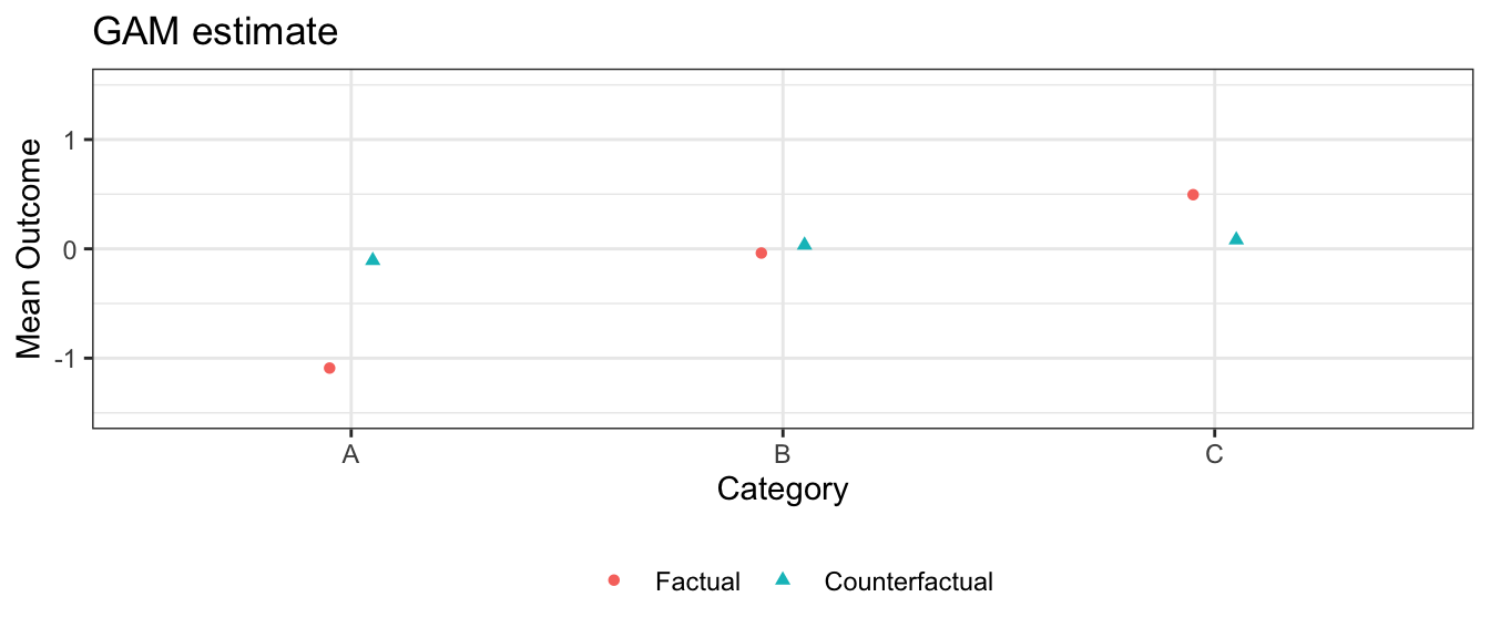
3.1 Generalized Additive Models

Perhaps you are concerned about linearity assumptions: the continuous confounder, for instance, might actually have a nonlinear association with the outcome. We know the truth is linear in this simulated example, but in practice you would never know. You can address this concern by estimating with a GAM, using the s() operator from mgcv for smooth terms (see Wood (2017)).

estimate_gam <- gapclosing(
  data = simulated_data,
  counterfactual_assignments = 1,
  outcome_formula = formula(outcome ~ s(confounder) + category*treatment),
  treatment_formula = formula(treatment ~ s(confounder) + category),
  category_name = "category",
  treatment_algorithm = "gam",
  outcome_algorithm = "gam",
  sample_split = "cross_fit"
  # Note: Standard errors with `se = TRUE` are supported.
  # They are omitted here only to speed vignette build time.
)

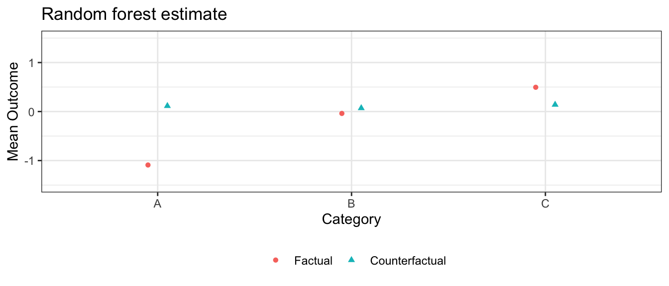
3.2 Random forests

Perhaps you are concerned that the true treatment probability and expected outcome functions have many interactions among the predictors. You can set treatment_algorithm and outcome_algorithm to “ranger” to estimate via the ranger function in the ranger package (Wright and Ziegler 2017).

One aspect of the way gapclosing() operationalizes ranger() is unique out of all the estimation algorithm options. When you choose a random forest, it is because you believe there are many important interactions. Some of the most important interactions may be between the treatment and the other predictors. Therefore, outcome_algorithm = ranger enforces those interactions by estimating the outcome model separately for treated and control units. For this reason, when outcome_algorithm = ranger there is no need to include the treatment variable explicitly in the outcome_formula.

estimate_ranger <- gapclosing(
  data = simulated_data,
  counterfactual_assignments = 1,
  outcome_formula = formula(outcome ~ confounder + category),
  treatment_formula = formula(treatment ~ confounder + category),
  category_name = "category",
  treatment_algorithm = "ranger",
  outcome_algorithm = "ranger",
  sample_split = "cross_fit"
  # Note: Standard errors with `se = TRUE` are supported.
  # They are omitted here only to speed vignette build time.
)

3.3 Estimates from these three algorithms are roughly the same

In this simulation, the GLM models are correctly specified and there are no nonlinearities or interactions for the machine learning approaches to learn. In this case, the sample size is large enough that those approaches correctly learn the linear functional form, and all three estimation strategies yield similar estimates.

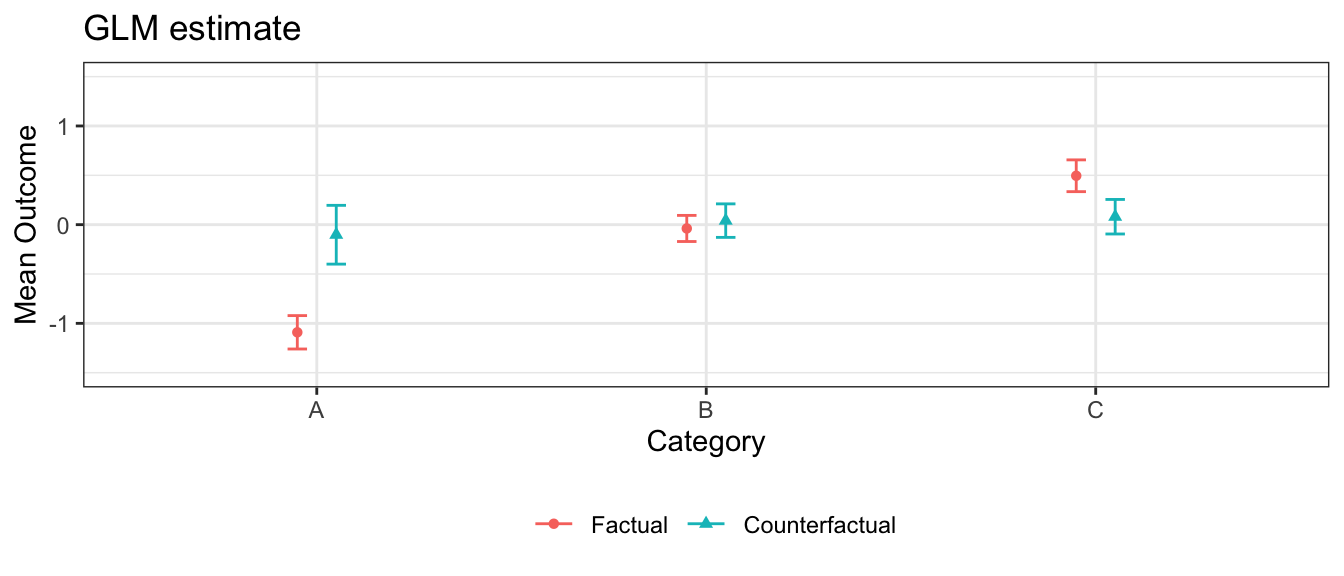
Note that confidence intervals for GAM and random forest can also be generated with SE = TRUE, which is turned off here only to speed vignette build time.

3.4 Word of warning

The assumptions of a parametric model are always doubtful, leading to a common question of whether one should always use a more flexible machine learning approach like ranger. In a very large sample, a flexible learner would likely be the correct choice. In the sample sizes of social science settings, the amount of data may sometimes be insufficient for these algorithms to discover a complex functional form. When the parametric assumptions are approximately true, the parametric estimators may have better performance in small sample sizes. What counts as “small” and “large” is difficult to say outside of any specific setting.