Causal Inference with Survival Outcomes
Review of causal inference
This material is taken from Soc 212B.
Fundamental problem of causal inference
Health professionals often advise people to eat a Mediterranean diet high in healthy fats such as olive oil, whole grains, and fruits. There is descriptive evidence that lifespans are longer among people who eat a Mediterranean diet compared with among people who eat a standard diet. But does eating a Mediterranean diet cause longer lifespan? The figure below visualizes this question in the potential outcomes framework.
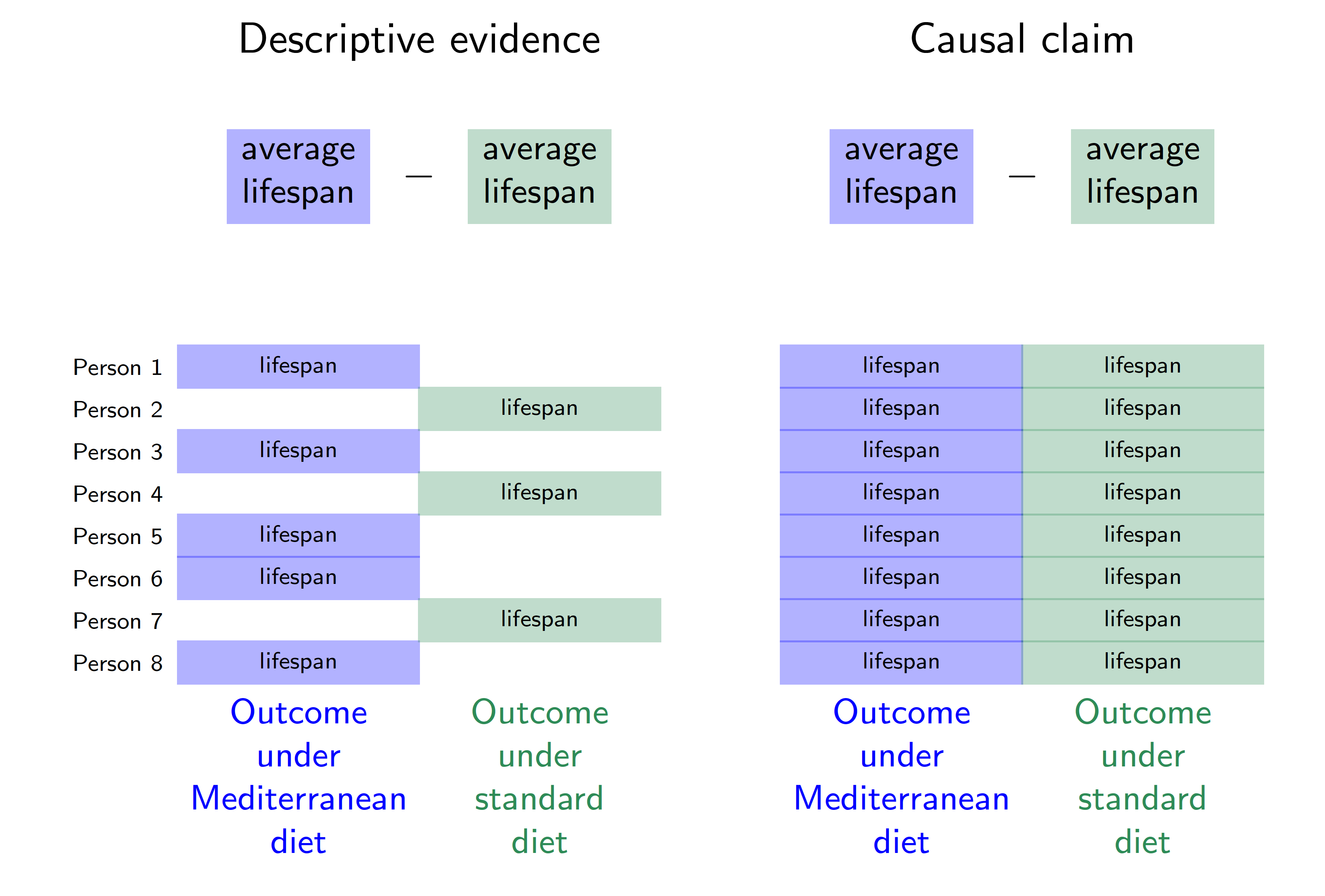
In this hypothetical example, each row corresponds to a person. Person 1 follows a Mediterranean diet and is observed to have a lifespan indicated in blue. Person 2 does not follow a Mediterranean diet and is observed to have a lifespan indicated in green. The descriptive evidence is that lifespans are longer among those eating a Mediterranean diet (blue outcomes on the left) compared with those eating standard diets (green outcomes on the left).
The right side of the figure corresponds to the causal claim, which is different. Person 1 has two potential outcomes: a lifespan that would be realized under a Mediterranean diet and a lifespan that would be realized under a standard diet. The causal effect for Person 1 is the difference between the lifespans that would be realized for that person under each of the two diets. But there is a fundamental problem: person 1 ate a Mediterranean diet, and we did not get to observe their outcome under a standard diet. The fundamental problem of causal inference (Holland 1986) is that causal claims involve a contrast between potential outcomes, but for each unit only one of these potential outcomes is realized. The other is counterfactual and cannot be directly observed.
We will need additional argument and assumptions to use the factual data (left side of the figure) in order to produce answers about causal effects (right side of the figure). Causal inference is a missing data problem insofar as many of the potential outcomes we need are missing.
Mathematical notation
Because each person has more than one potential outcome, we need new mathematical notation to formalize causal claims. We will use subscripts to indicate units (rows of our data). Let \(Y_i\) be the outcome for person \(i\), such as whether person \(i\) survived. Let \(A_i\) be the treatment of person \(i\), for example taking the value or the value . To refer more abstractly to a value the treatment could take, we use the lower case notation \(a\) for a treatment value. Define potential outcomes \(Y_i^\text{MediterraneanDiet}\) and \(Y_i^\text{StandardDiet}\) as the lifespan outcomes that person \(i\) would realize under each of the treatment conditions. More generally, let \(Y_i^a\) denote the potential outcome for unit \(i\) that would be realized if assigned to treatment value \(a\).
The causal effect is a contrast across potential outcomes. For example, the causal effect on Ian’s lifespan of eating a Mediterranean diet versus a standard diet is \[Y_\text{Ian}^\text{MediterraneanDiet} - Y_\text{Ian}^\text{StandardDiet}\]
To connect causal claims to ideas we have already covered from sampling, we will adopt a framework in which potential outcomes are fixed quantities with randomness arising from sampling and/or from random treatment assignment. Each person has a fixed outcome \(Y_i^\text{MediterraneanDiet}\) that would be observed if they were sampled and assigned a Mediterranean diet. This is just like how every baseball player from last week had a salary that would be observed if they were sampled. We will sometimes omit the \(i\) subscript to refer to the random variable for the potential outcome of a randomly-sampled person from the population, \(Y^\text{MediterraneanDiet}\).
Survival outcomes: What changes?
What is different for survival outcomes? In some sense, very little changes. At time \(t = 0\), each participant \(i\) is randomized to the treatment \(A_i = 0\) or \(A_i = 1\). We might define survival \(Y_i\) as the time since that point until death.
Very little has changed. Given that you already know survival models, one trivial change is that there may be censoring: some people drop out of the study (\(C_i = 1)\) before death. But under ignorable censoring, this change is easily solved by using Kaplan-Meier or a parametric survival model like the Weibull. Simply estimate survival curves in the treated and untreated groups.
In a simple and well-designed study, nothing else changes. But in many realistic settings, causal inference for survival outcomes brings additional care that must be placed on the alignment of the clock.
Clock seems to start before treatment
When setting up a survival analysis, one of the first questions is what time should be time zero. The wrong choice can make your causal inference much more complicated, as we illustrate through an example.
A set of \(n\) patients diagnosed with a type of cancer at time \(t\) are enrolled in a study. At a later time point \(t'>t\), those who are still alive are randomized to an experimental treatment \(A_i = 1\) or to the existing standard of care \(A_i = 0\). A researcher then studies the causal effect of the treatment on survival time \(Y_i\).
For defining survival time \(Y_i\), how should the researcher define time 0?
- Survival since birth
- Survival since diagnosis (time 0 = \(t\))
- Survival since treatment assignment (time 0 = \(t'\))
The answer is (c): you should define survival since the time of treatment assignment. The treatment effect is how treatment affects survival after it is implemented.
What goes wrong under (a) or (b)? Some patients die between time 0 and the time treatment is assigned. These patients must be dropped from the study because they do not have treatment values. A consequence of this is known as immortal time bias: during the time from time 0 to time \(t'\), no one in the study can die (see Hernan et al. 2016 and 2025).
Clock seems to start after treatment
Ideally, the clock starts at the time of treatment. But what if the most reasonable place for the clock to start seems to be a time long after treatment? This can lead to other problems.
As an example, consider a demographer who studies the causal effect of a college degree (\(A_i\)) on the duration of first marriages (\(Y_i\)). The demographer restricts the sample to those who marry and starts the clock at the time when the first marriage begins.
What goes wrong with the clock in the example above? Think about
- who is eligible for the study
- how is time 0 defined for each of them
For simplicity, you may
- assume that no one marries until their education is completed
- assume that you are able to randomly assign college degrees to those eligible for the study
Suppose all high school graduates are eligible for the study. You randomly assign some to college degrees (\(A_i = 1\)) and others to stop education after high school (\(A_i = 0\)). You may be tempted to start the clock at entry into first marriage. But only some of the people go on to become married: say \(M_i=1\) if enters first marriage and \(M_i = 0\) otherwise. Time zero is only defined for \(M_i = 1\). What is worse, it is plausible that the value of \(M_i\) is itself shaped by the treatment.
What should these researchers do? There are at least two options.
Option: Redefine the outcome
Let the clock start at age 25. Define education (\(A_i\)) at age 25. Define time to event \(Y_i\) as the time until a first marriage ends or death, whichever is sooner. Now every person has a time 0 and an outcome. But you are no longer studying duration of first marriage; you are now studying age of marital dissolution or death.
Option: Mediation estimands
Let \(Y_i^{a,m = 1}\) be the marital duration that person \(i\) would experience if assigned to education value \(A_i = a\) and assigned to enter a first marriage (\(M_i = m = 1\)). Then all people have a marital duration \(Y_i^{a,m_i=1}\) that would be realized under each treatment value \(a\). The causal estimand might be a controlled direct effect,
\[ \text{P}(Y^{a=1,m=1} > t) - \text{P}(Y^{a=0,m=1} > t) \]
which is the causal effect of a college degree (\(a = 1\) vs \(a = 0\)) on first marriage survival longer than \(t\) in a world where everyone is assigned to enter a first marriage (\(m = 1\)).
A future page will introduce methods to estimate this estimand in observational settings.
Option: Principal stratification estimands
In theory, one could define the latent subpopulation who would get married under either treatment assignment: \(M_i^{a=0}=M_i^{a=1}=1\). One can then use principal stratification to set-identify the causal effect of treatment on first marriage duration in this latent set.
\[ \text{P}(Y^{a=1} > t\mid M^{a=0}=M^{a=1}=1) - \text{P}(Y^{a=0,m=1} > t\mid M^{a=0}=M^{a=1}=1) \]
This is a somewhat complicated estimand with a complicated estimation strategy. We will not cover it in class (though I am working on a paper about this estimand).
Next pages will be: Observational studies. Mediation.