Proportional Hazards

Many models we have already learned are examples of a broader model class called proportional hazards models. These models begin with a baseline hazard that applies when \(\vec{X} = \vec{0}\). For other values of \(\vec{X}\), the hazard equals the baseline hazard multiplied by hazard ratio \(e^{\vec{X}'\vec\beta}\).

\[ h(t\mid\vec{X}) = \underbrace{\lambda(t)}_{\substack{\text{baseline}\\\text{hazard}}}\underbrace{e^{\vec{X}'\vec\beta}}_{\substack{\text{hazard}\\\text{ratio}}} \]

Let’s see proportional hazards in a concrete example. On the Weibull page, we created an object predicted_survival containing the predicted values of a survival curve. Below, we load this object again.

predicted_survival <- read_csv("assets/predicted_survival_weibull.csv")

Recall that this object has two units with x = 0 and x = 1, with many rows per unit representing survival probabilities at each time point. We can calculate the hazard at these time points as well.

predicted_hazard <- predicted_survival |>
  mutate(
    # Calculate the PDF at each point
    f = dweibull(x = time, shape = shape, scale = scale),
    # Hazard equals PDF over survival
    h = f / S
  )

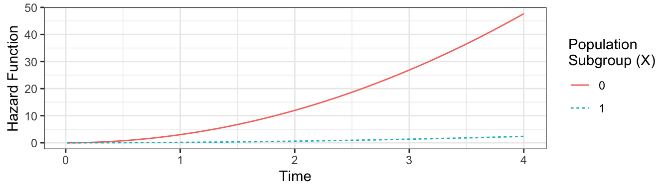
Below we visualize these hazard functions. The hazard in population subgroup \(X = 0\) is much higher than the hazard in subgroup \(X = 1\), at every time point.

Code

predicted_hazard |>
  select(x, time, h) |>
  ggplot(aes(x = time, y = h, color = factor(x), linetype = factor(x))) +
  geom_line() +
  labs(
    y = "Hazard Function", 
    x = "Time", 
    color = "Population\nSubgroup (X)",
    linetype = "Population\nSubgroup (X)"
  )

Next, consider the hazard ratio at each time \(t\): the hazard in group \(X = 1\) divided by the hazard in group \(X = 0\).

Code

predicted_hazard_ratios <- predicted_hazard |>
  select(x, time, h) |>
  pivot_wider(names_from = "x", values_from = "h", names_prefix = "hazard_if_x_") |>
  mutate(hazard_ratio = hazard_if_x_1 / hazard_if_x_0) |>
  print(n = 5)

# A tibble: 100 × 4
    time hazard_if_x_0 hazard_if_x_1 hazard_ratio
   <dbl>         <dbl>         <dbl>        <dbl>
1 0.01        0.000309     0.0000153       0.0496
2 0.0503      0.00774      0.000384        0.0496
3 0.0906      0.0250       0.00124         0.0496
4 0.131       0.0521       0.00259         0.0496
5 0.171       0.0890       0.00442         0.0496
# ℹ 95 more rows

Note that the hazard ratio is constant in this model. The hazard ratio is 0.0496 at every time point. A hazard ratio that is constant over time is the hallmark of a proportional hazards model: the hazard function at every \(\vec{x}\) value is proportional to a baseline hazard that exists if \(\vec{x} = \vec{0}\).

Math for Exponential and Weibull PH

Here we use math to see the Exponential and Weibull models as proportional hazards models.

Exponential PH in math

For the Exponential model \(T\sim\text{Exponential}(\lambda)\) with where we model the rate parameter \(\lambda = \exp(\beta_0 + \beta_1 X)\), the hazard function is \(h(t) = \lambda = \exp(\beta_0 + \beta_1 X)\). The baseline hazard when \(X = 0\) is \(\exp(\beta_0)\), and the hazard when \(X = 1\) is \(\exp(\beta_0 + \beta_1)\). The hazard ratio for \(X = 1\) vs \(X = 0\) is \(\exp(\beta_1)\).

Weibull PH in math

For a Weibull with shape \(\alpha\) and scale \(\sigma\), the probability density function is \[ f(t) = \alpha \sigma ^ {-\alpha} t^{\alpha-1}e^{-(\frac{1}{\sigma} t)^\alpha} \] and the survival function is \[ S(t) = e^{-(\frac{1}{\sigma} t)^{\alpha}} \] Taking the ratio, the hazard function is

\[ h(t) = \alpha \sigma ^ {-\alpha} t^{\alpha-1} \]

When using the survreg function in the survival package, we model \(\sigma = \exp(\beta_0 + \beta_1 X)\). Plugging this in, we can see how the Weibull hazard function is proportional across values of \(X\).

\[ \begin{aligned} h(t) &= \alpha \left(e^{\beta_0 + \beta_1 X}\right) ^ {-\alpha} t^{\alpha-1} \\ &= \underbrace{\alpha e^{-\alpha\beta_0}t^{\alpha - 1}}_{\substack{\text{baseline}\\\text{hazard}}}\underbrace{e^{\beta_1 X}}_{\substack{\text{hazard}\\\text{ratio}}} \\ &= \begin{cases} \alpha e^{-\alpha\beta_0}t^{\alpha - 1} &\text{if }x=0 \\ \alpha e^{-\alpha\beta_0}t^{\alpha - 1}e^{-\alpha\beta_1} &\text{if }x=1 \end{cases} \end{aligned} \]

We can confirm that this hazard ratio is correct in the fitted model (see the Weibull page for fitting this model).

model <- readRDS("https://ilundberg.github.io/eventhistory/assets/weibull_model.RDS")

alpha_hat <- 1 / model$scale
beta1_hat <- coef(model)[2]
hazard_ratio <- exp(- alpha_hat * beta1_hat)

The resulting hazard ratio 0.0496 is equal to the one we calculated from predicted values 0.0496. Thus, our mathematical understanding of the Weibull proportional hazards model aligns with the predicted values from the canned output.