Competing Risks

We have generally assumed ignorable censoring: at any time point \(t\), the probability of becoming censored is the same for all units who are alive at that time point, regardless of their future time until death.

Another way to think about ignorable censoring is to let \(C\) be the time until censoring and \(T\) be the time until the event of interest. Then we assume \(C\) is independent of \(T\). A unit is censored if it happens that \(C < T\), and a unit has the event if \(T \leq C\).

Competing risks are a common setting that violates the assumption of ignorable censoring. We will consider competing risks through a concrete example.

Illustration: Retirement and death

This example comes from an example that German Rodriguez developed about the retirments and deaths of Supreme Court justices. Here is the original source. He used Wikipedia and the Supreme Court website to create a dataset on the time that Supreme Court justices were in office, and how their time ended (retirement, resignation, death, still an incumbent). The code at the button below takes his data and simplifies them for our analysis.

retirement <- read_csv("https://grodri.github.io/datasets/justices.csv") |>
  mutate(
    start = parse_date(startstr, format = "%B %d, %Y"),
    stop = parse_date(stopstr, format = "%B %d, %Y"),
    # Make t time on the bench in days
    t = difftime(stop, start, units = "days"),
    # Convert to years
    t = as.numeric(t) / 365.25,
    age_appointed = as.numeric(difftime(
      stop,
      parse_date(birthstr, format = "%B %d, %Y"),
      units = "days"
    )) / 365.25
  ) |>
  # Keep only those who died or resigned
  filter(status != "Incumbent") |>
  select(number, name, state, age_appointed, status, t) |>
  write_csv("assets/retirement.csv")

You can load the simplified data retirement.csv directly with the line below.

retirement <- read_csv("https://ilundberg.github.io/eventhistory/assets/retirement.csv")

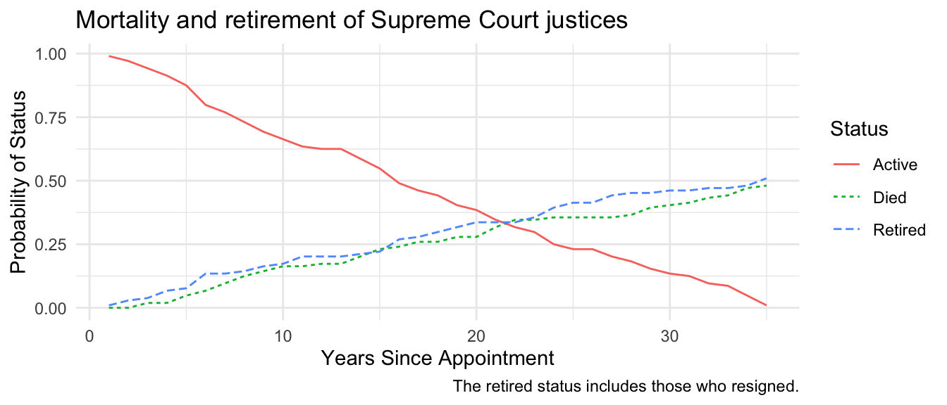
Initially, the justices are all active. Over time since appointment, they gradually move into one of two final states: either death (status = "Died") or retirement (status = "Resigned" or status = "Retired").

library(foreach)
by_years <- foreach(years_val = 1:35, .combine = "rbind") %do% {
  tibble(
    years = years_val,
    active = mean(retirement$t > years_val),
    retired = mean(retirement$t <= years_val & retirement$status %in% c("Resigned","Retired")),
    died = mean(retirement$t <= years_val & retirement$status == "Died")
  )
}
by_years |>
  pivot_longer(cols = -years, names_to = "status") |>
  ggplot(aes(x = years, y = value, color = status, linetype = status)) +
  geom_line() +
  labs(
    x = "Years Since Appointment",
    y = "Probability of Status",
    color = "Status",
    linetype = "Status",
    title = "Mortality and retirement of Supreme Court justices",
    caption = "The retired status includes those who resigned."
  ) +
  scale_color_discrete(labels = stringr::str_to_sentence) +
  scale_linetype_discrete(labels = stringr::str_to_sentence)

Death and retirement happen at remarkably similar rates over time!

A Kaplan-Meier estimate of survival

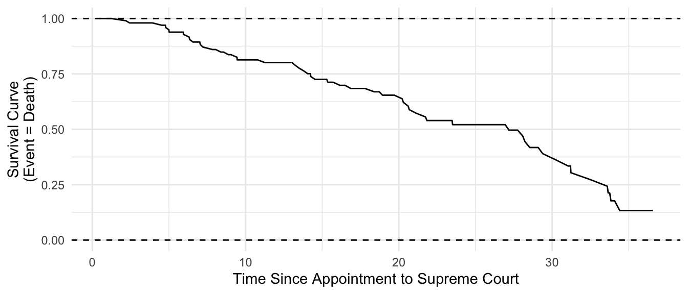
Suppose death is the event of interest. The data only contain death dates for those who died in office; otherwise we only know that the justice was alive until they retired. We might estimate survival as a function of time since appointment by Kaplan-Meier, where censoring is retirment and the event is death.

km <- survfit(
  Surv(t, event = status == "Died") ~ 1, 
  data = retirement
)

The figure below visualizes the resulting survival curve.

km |>
  broom::tidy() |>
  ggplot(aes(x = time, y = estimate)) +
  geom_hline(yintercept = c(0,1), linetype = "dashed") +
  geom_line() +
  labs(
    y = "Survival Curve\n(Event = Death)",
    x = "Time Since Appointment to Supreme Court"
  )

Notice the right end of this curve. The Kaplan-Meier estimates show that justices have a 12.5% chance of living for 35 years after appointment! Given that the median age at appointment is 71, this means that the median justice has a 12.5% chance of surviving past the age of 106. Surely this is misleading!

What has gone wrong

The problem here is that censoring (retirement) is not independent of the event of interest (death). Supreme Court justices often serve on the bench until their health is poor. If we imagine a justice who has served 20 years on the bench and then retires, that justice’s hazard of death is likely higher than the hazard for another justice who has served 20 years on the bench and continues to serve. But Kaplan-Meier (and all survival models) has assumed that censoring is independent of the hazard of death.

What to do

Non-ignorable censoring is a deep problem, and easy answers are elusive. There exist multivariate survival models that assume a correlation between the latent risks of multiple distinct hazards. But these models come with their own assumptions and can be difficult to explain to a reader.

In the presence of competing risks, one simple solution is to visualize all the competing risks, as in the figure at the top of this page. This may be a good practice in applied research.