nlsy_outcomes <- read_csv("https://ilundberg.github.io/eventhistory/assets/nlsy_outcomes.csv")Data
This page is a reference for several datasets that we use in the course.
Four life outcomes
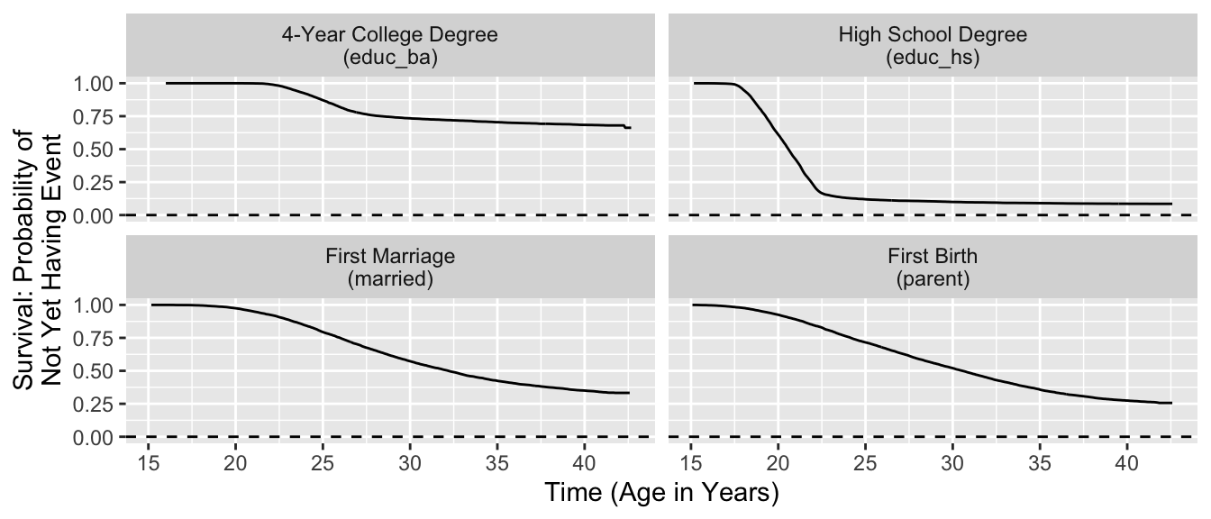
The file nlsy_outcomes.csv contains data from the NLSY97 cross-sectional sample (excluding oversamples). Each person (indexed by id) has four rows corresponding to four outcomes: high school completion, BA completion, marriage, and first birth.
idis the person identifiersexis a covariate from the baseline interviewraceis a covariate from the baseline interviewoutcomeis the outcome that the row summarizes:educ_hsfor high school completion,educ_bafor college,marriedfor first marriage, andparentfor first birthtimeis the age in years at which the outcome occurs, or the unit is censoredcensoredis an indicator variable codedFALSEif the outcome occurs andTRUEif the unit was censored: the last interview happened without the event occurring. For units withcensored = TRUE, thetimevariable is the age at the last interview.
When analyzing these data, you should first filter the data to a single value of outcome that you plan to study. The figure below shows Kaplan-Meier survival curves for these four outcomes.
Employment duration
This dataset can be used to model the duration of an employment spell as a function of covariates defined at the beginning of the spell.
The file employment_duration.csv contains data from the NLSY97 cross-sectional sample (excluding oversamples). Each row is a (person \(\times\) employment spell). Variables are defined as follows:
idis a person identifiertimeis the duration of the employment spell in years. It begins with the month a respondent moves from being non-employed to being employed at least one week. It ends with the month a respondent becomes non-employed again for an entire month.censoredis an indicator for being censored, codedTRUEif the last interview occurred during this employment spell andFALSEif the end of the employment spell was observed- Two covariates are defined at the baseline survey:
sexandrace - Four covariates are defined at the start of the employment spell:
age,education,marital, andparent(whether the respondent is a parent)
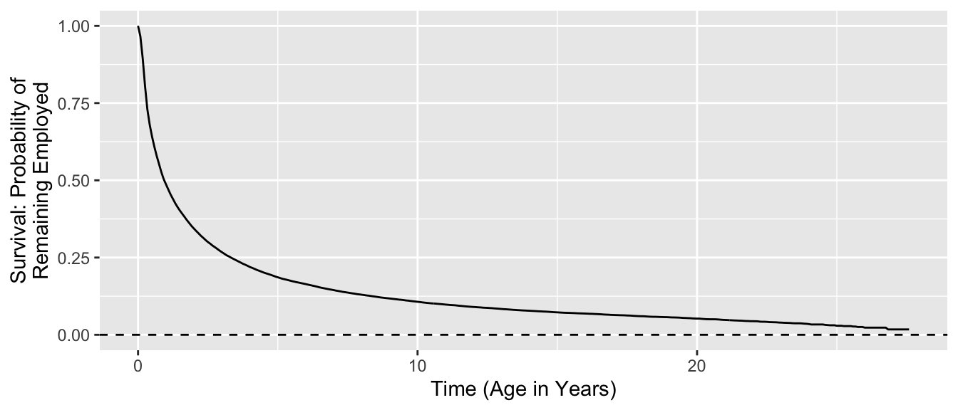
employment_duration <- read_csv("https://ilundberg.github.io/eventhistory/assets/employment_duration.csv")The figure below shows a Kaplan-Meier survival curve for first marriage duration in these data.
First marriage duration
This dataset can be used to model the duration of a first marriage as a function of covariates defined at the beginning of the marriage. It can also be used to reason about competing risks, because marriages end for several reasons recorded in the how_end variable.
The file first_marriage_duration.csv contains data from the NLSY97 cross-sectional sample (excluding oversamples). Each row is a person who reports the start of a first marriage.
idis a person identifiercensoredis an indicator for being censored, codedTRUEif the last interview occurred while the respondent was still married andFALSEif otherwise (i.e., end of marriage was observed)timeis the duration of the first marriage in years, until either the end of the marriage or censoringhow_endis how the marriage ended:Censored,Divorced,Legally Separated, orWidowed- Two covariates are defined at the baseline survey:
sexandrace - Three covariates are defined at the start of the first marriage:
age,education, andparent(whether the respondent is a parent)
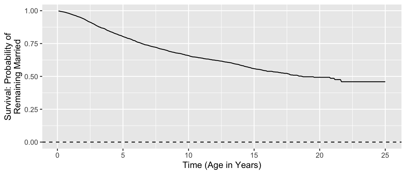
first_marriage_duration <- read_csv("https://ilundberg.github.io/eventhistory/assets/first_marriage_duration.csv")The figure below shows a Kaplan-Meier survival curve for first marriage duration in these data.
U.S. life table deaths
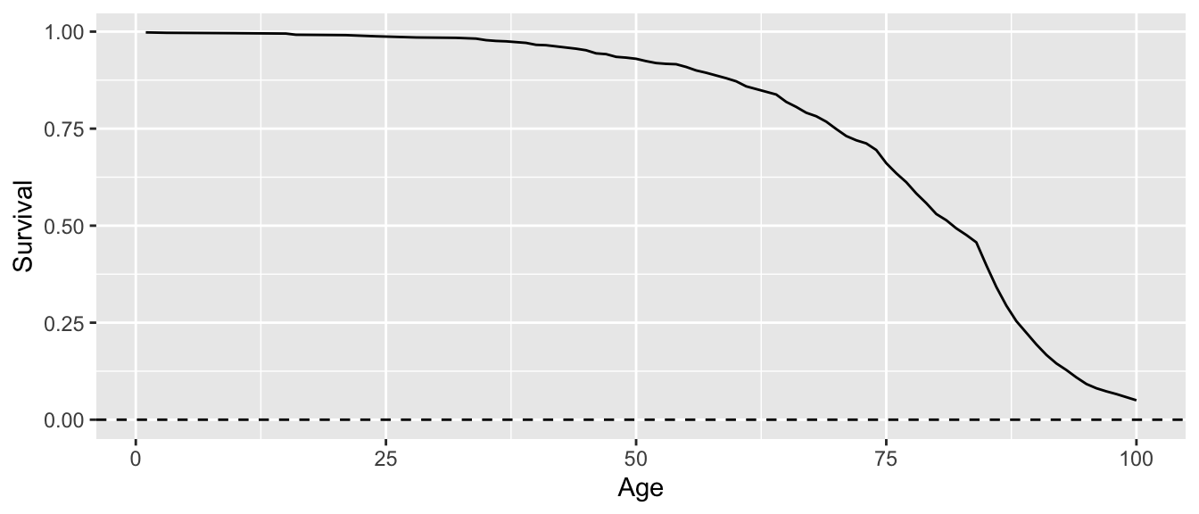
Using 2023 U.S. age-specific mortality data from an NCHS report, I generated deaths for a hypothetical population that experiences these rates, available in deaths.csv.
deaths <- read_csv("https://ilundberg.github.io/eventhistory/assets/deaths.csv")These data include
idindexes simulated personsageis the time variablediedis whether the person died (died = 1) or was censored (died = 0)
The figure below visualizes Kaplan-Meier survival estimates in these data.
Heart recipients
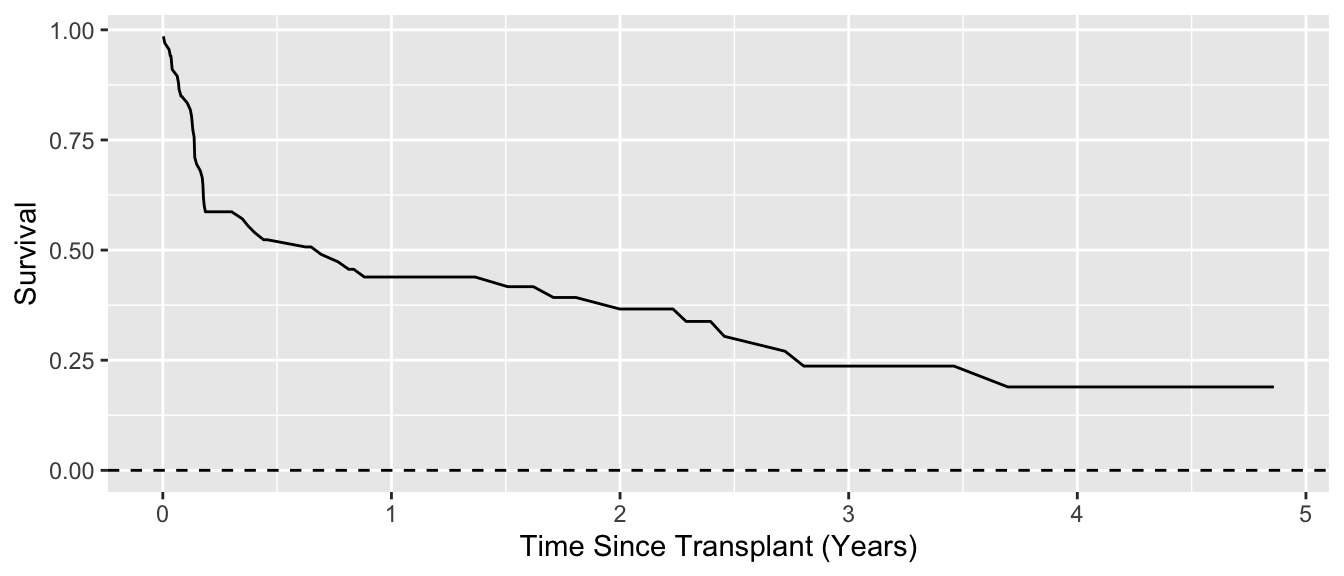
These data come from a medical trial that tracked survival outcomes of patients receiving heart transplants.
Crowley, J., & Hu, M. (1977). Covariance analysis of heart transplant survival data. Journal of the American Statistical Association, 72(357), 27-36.
The trail enrolled people eligible for heart transplants, some of whom later received transplants and some did not. The full data are available in the jasa data object of the survival package. A simplified version of the data focuses on survival outcomes post-transplant for transplant recipients. This simplified file is heart_recipients.csv.
heart_recipients <- read_csv("https://ilundberg.github.io/eventhistory/assets/heart_recipients.csv")In the heart_recipients data,
tis time in years from transplant until either death or censoringcis censoring, codedTRUEfor censoring andFALSEfor deathageis the patient’s age at the time of transplant
Below is a Kaplan-Meier survival curve with these data.
Justice retirement
These data were originally collected by German Rodriguez (original source). He used Wikipedia and the Supreme Court website to create a dataset on the time that Supreme Court justices were in office, and how their time ended (retirement, resignation, death, still an incumbent).
A simplified version of these data is retirement.csv
retirement <- read_csv("https://ilundberg.github.io/eventhistory/assets/retirement.csv")These data contain
numberindexes Supreme Court justicesnamecontains namesstatecontains the justice’s home stateage_appointedis the age at which the justice was appointedstatusindicates how the term ended (Resigned,Retired, orDied)tis the total time from appointment untilstatus
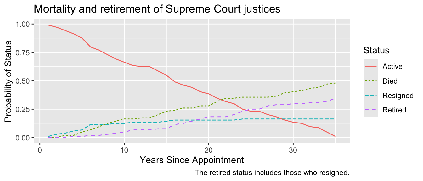
The graph below shows the cumulative proportion in each status over time.