employment_duration <- read_csv("https://ilundberg.github.io/eventhistory/assets/employment_duration.csv")Problem Sets
Problem sets are currently posted on Piazza, but I plan to gather them on this page.
Problem Set 1: Key Concepts
A study enrolls 6 people looking for work. 3 are randomly assigned to a job training intervention and 3 are randomly assigned to no job training. Over a 52-week follow-up period beginning January 1, the study records the time until they are hired in weeks.
| ID | Age | Treatment | Time until hired |
|---|---|---|---|
| 1 | 53 | Treated | 12 weeks |
| 2 | 26 | Treated | 10 weeks |
| 3 | 37 | Treated | 44 weeks |
| 4 | 25 | Untreated | 7 weeks |
| 5 | 48 | Untreated | Never hired in 52 weeks |
| 6 | 34 | Untreated | 40 weeks |
- What is time 0 in this study?
- Which unit(s) were censored?
- Can you point identify the mean time until hired in the treatment condition? If not, can you provide a lower bound? Ignore statistical uncertainty.
- Can you point identify the mean time until hired in the untreated condition? If not, can you provide a lower bound? Ignore statistical uncertainty.
- Does the job training reduce the average time until hired?
The next questions are about the Exponential distribution, which assumes a constant hazard: \(h(t) = \lambda\).
- True or False. The CDF \(F(t) = P(T < t)\) is an increasing function of \(t\).
- True or False. The survival function \(S(t) = P(T > t)\) is an increasing function of \(t\).
- A demographer studies a cohort of people born in 1965 where age is the time variable (with time zero at age zero). They study the time until first marriage. In 1–3 sentences, make an argument that the assumption of a constant hazard is implausible.
Problem Set 2: Exponential
See the exercise at the end of the Exponential page.
Problem Set 3: Weibull
This problem set practices Kaplan-Meier survival curve estimation and a Weibull model.
The survival::veteran data contain data from a clinical trial involving cancer patients run by the Veteran’s Administration. These data are described in Kalbfleisch and Prentice (1980) on p.~60. There are 137 patients, and only 9 are censored before death.
statusis 1 for death, 0 for censoringtimeis days of survivaltrtis a randomized chemotherapy test treatment. 1 indicates standard treatment, 2 indicates the test treatment
For more information on the data see ?survival::veteran.
- (10 points) Estimate survival curves by treatment status
trt, using the Kaplan-Meier method. Visualize the results in a plot. - (10 points) Estimate survival curves by treatment status
trt, using a Weibull regression with only this predictor. Visualize the results in a plot. - (10 points) Compare: Plot the Weibull and Kaplan-Meier survival curves on the same plot. How do they differ? For ease of comparison, you might use different panels or different plots for each treatment status so that it is easier to compare across models within treatment status.
- (10 points) Plot the estimated Weibull hazard function. Does it increase or decrease with time?
- (8 points) In your Weibull results, can you reject the null of an Exponential model?
- (2 points, Challenge): Construct a confidence interval on each point of your Weibull survival functions and visualize the result. Note that this is quite challenging; it is only worth 2 points so that you can skip it and still get an A on the problem set. Here are some steps.
- Define the X matrix at which to make predictions
- Loop over simulations. In each iteration,
- Simulate \(\vec\beta\) and the
log_scaleparameter from a Multivariate Normal centered atc(coef(model), log(model$scale))with variance-covariance matrixvcov(model) - Calculate the simulated value of the
rweibullparameterscale, which is \(e^{\vec{X}'\vec\beta}\) where \(\vec\beta\) are coefficients fromsurvreg - Calculate the simulated value of the
rweibullparametershape, which is1 / exp(log_scale)wherelog_scaleis the simulated value of the log of whatsurvregcalls the scale parameter - Simulate survival functions with those parameters
- Simulate \(\vec\beta\) and the
- At each point of the survival curve, calculate the 2.5 and 97.5 percentiles of the empirical distribution of simulated draws.
Problem Set 4: Recap of Survival Analysis
This problem set asks you to carry out a survival analysis of your choosing using concepts we have learned in the course. Choose one of the NLSY datasets on the data page, which include
- nlsy_outcomes.csv which contains time to high school completion, college completion, marriage, and parenthood with a few basic covariates
- In this dataset, you would likely choose 1 of the 4 outcomes
- employment_duration.csv which contains the duration of spells of employment, with many covariates defined at the start of the spell
- first_marriage_duration.csv which contains the duration of first marriages, with many covariates defined at the start of the spell
Below are the questions for the problem set.
- Define time 0, time to event, and censoring for your question.
- Visualize survival with Kaplan-Meier. Interpret something about the estimated curve.
- Using one or more covariates and a model with a parametric hazard, compare survival curves across subgroups.
- Explain why you made your particular modeling choices.
- In words, give an example of non-ignorable censoring that could exist in your setting.
- In words, give an example of unmeasured heterogeneity that could exist in your setting. How might this affect the estimated hazard function?
Problem Set 5: Causal Effect on Survival
The file employment_duration.csv contains information on spells of employment.
At the start of each employment spell, we observe whether the respondent works fulltime = TRUE or fulltime = FALSE, where fulltime is an indicator of working 40+ hours in at least one week during the first month of the job. This problem set considers a causal question: to what degree does being employed full-time at the start affect the length of the employment spell?
We will make the simplifying assumptions of ignorable censoring and that selection on observables holds conditional on the following confounder set: race, sex, age, and education.
As context, below are the descriptive Kaplan-Meier survival curves by full-time status (with no confounder adjustment).
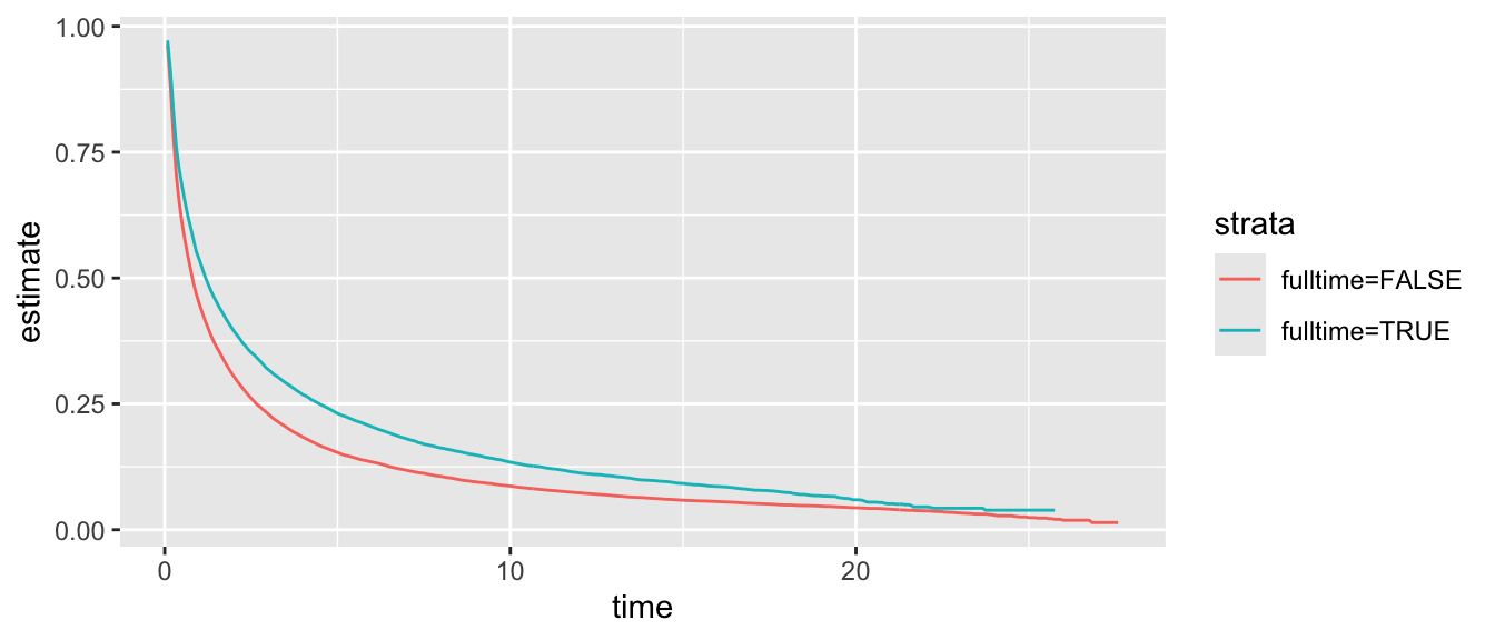
As a concrete data point, the probability of remaining employed for 5 years among those in each treatment group is given below. There is approximately an 8 percentage point difference across treatment conditions.
# A tibble: 2 × 2
# Groups:   Treatment_Value [2]
  Treatment_Value Survives_5_Years
  <chr>                      <dbl>
1 fulltime=FALSE             0.154
2 fulltime=TRUE              0.231
Estimate a Weibull model for employment duration as a function of the treatment
fulltimeand the confoundersrace,sex,age, andeducation.Create two new data frames to make predictions. Each begins as
employment_duration. In the first data frame, setfulltime = TRUEfor all cases. In the second data frame, setfulltime = FALSEfor all cases.In each data frame, use your model to predict the probability of surviving (remaining in the employment spell) for at least 5 years, for every person in the data frame.
Take the average of the predicted probabilities. These are estimates of \(\text{P}(Y^{\text{fulltime} = \text{TRUE}} > 5)\) and \(\text{P}(Y^{\text{fulltime} = \text{FALSE}} > 5)\). Report each estimate and the difference between them, which is your estimated causal effect. How does it compare to the 8 percentage point descriptive difference?
Note. This is not part of the assignment because we have already practiced it previously, but worth noting. You can imagine running a loop over many time points and then creating counterfactual survival curves for the population-average survival in each counterfactual scenario. The problem set just chose one time point (time = 5) for illustration.
Problem Set 6: Longitudinal Treatments
A researcher wants to know the expected potential outcome \(\text{E}(Y^{a_0,a_1})\) under an intervention to set \(A_0 = a_0\) and \(A_1 = a_1\). Assume that variables named \(A,L,Y\) are observed but variables named \(U\) are unobserved.
- In which of settings A–D can this causal estimand be identified using the simple mean \(\text{E}(Y\mid A_0 = a_0, A_1 = a_1)\)?
- In which of settings A–D can this causal estimand be identified using inverse probability weights applied in a marginal structural model, adjusting at each period for the observed past?
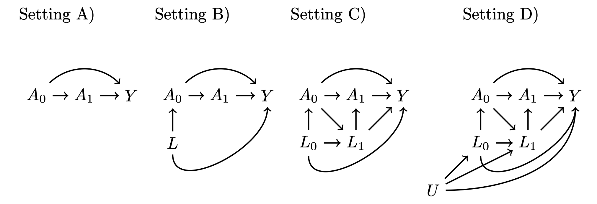
- Now focus on Setting D. For Setting D, explain how \(L_1\) complicates the quest to identify the effect of \(A_0\) and the effect of \(A_1\) with the same adjustment set for both effects.
The next part practices estimating a marginal structural model in a dynamic setting designed to be as simple as possible.
Suppose a teacher observes students who are struggling academically (\(L_t = 1\)) or not (\(L_t = 0)\) in every time period \(t\). The teacher can assign students to receive extra support (\(A_t = 1\)) or not (\(A_t = 0\)). The outcome \(Y\) is a subsequent measure of skills (e.g., can the student read a picture book to the teacher). The data pset6.csv contains a simulated setting with \(n = 128\) students.
In this data generating process,
- Treatment \(A_t = 1\) is assigned with higher probabilities to students who are struggling \(L_t = 1\).
- Students who are treated in one period \(A_0 = 1\) are never struggling in the next period \(L_1 = 0\).
Assume the causal structure represented by Setting D above. Using these data,
- Fit a logistic regression for each \(A_t\), including as predictors all pre-treatment variables entered without interactions.
- Predict the probability of \(A_t = 1\) at each time period for every unit. Remember that in R you will need the
type = "response"option. For grading, what is the predicted probability of \(A_0\) for the first unit in the sample? - Define the generalized propensity score \(\pi_{it}\) at each time period \(t\) for each unit \(i\). When \(A_{it}=1\), this is the probability of treatment. When \(A_{it}=0\), this is the probability of being untreated.
- Define a weight for each unit: \(w_i = \frac{1}{\pi_{i0}}\frac{1}{\pi_{i1}}\). For grading, what is the weight on the first unit in the sample?
- Estimate a marginal structural model of the form \(\text{E}(Y^{a_0,a_1}) = \alpha + \beta_0 a_0 + \beta_1 a_1\). Report the coefficients.
- What does your model estimate for the average causal effect \(\text{E}(Y^{1,1} - Y^{0,0})\)?
Problem Set 7: Course wrap-up
This problem set is a chance to reflect on the course and how it connects to your research. It is also a chance for me to gather feedback about what works well and what could be improved in the course.
- What is an example of an event history problem in your research area? This could involve a time-to-event outcome or a sequence of events as treatments. How might you use a method from this course to answer that question?
- Think of a statistical concept you did not know before this quarter that you now understand. What was that concept? Why do you think it particularly stuck with you? Are there ways the course design made that concept easier to learn?
- Is there a concept from the course that you wish you understood better? Do you have ideas for how we could cover that concept better when this course is taught again?