Weibull

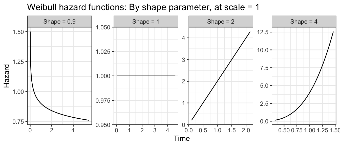
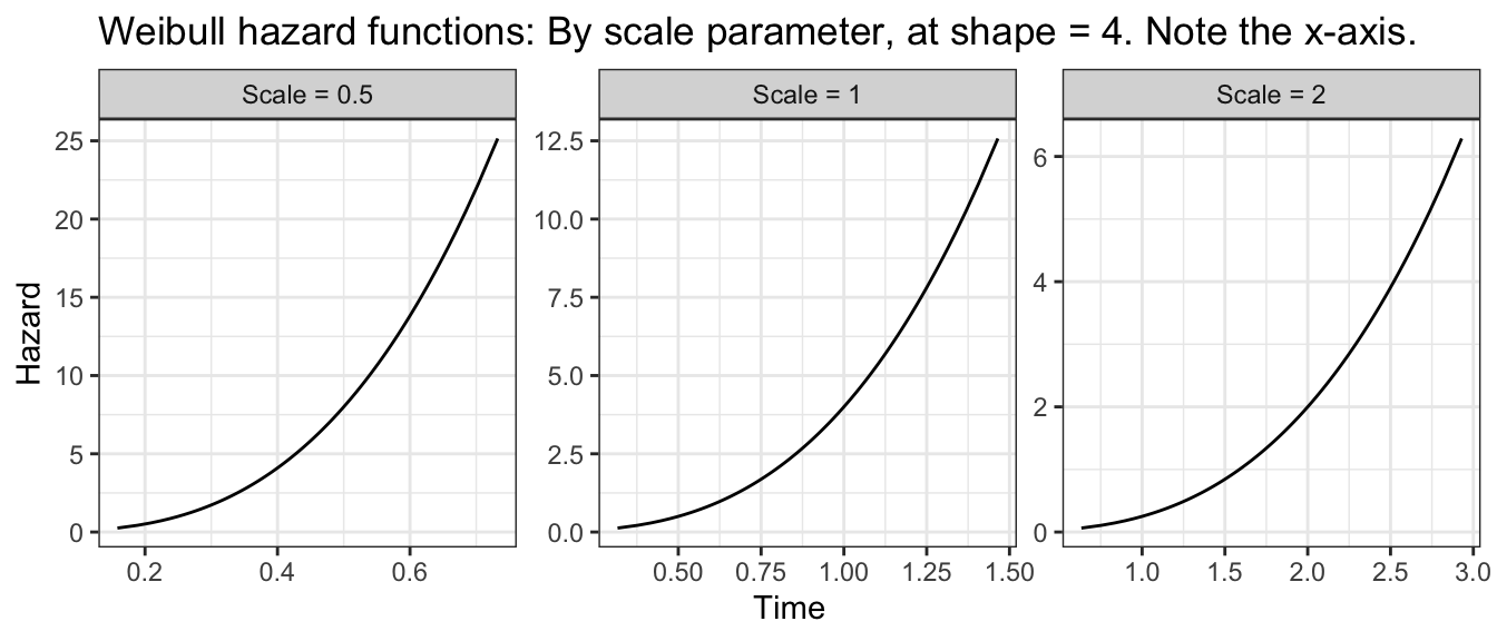
Like the Exponential, the Weibull is a distribution defined on positive real numbers. The Weibull is commonly used in survival analysis because it produces a hazard function that can increase with time or decrease with time. The Weibull hazard is always monotonic (either always increasing or always decreasing, or flat). The distribution functions in R are *weibull with * being d, r, q, or p.

These functions parameterize the Weibull with two parameters: shape and scale.

The shape determines how the hazard function changes with time. Below are Weibull hazards with several shape parameters and with fixed scale = 1.

Code

foreach(shape_value = c(.9,1,2,4), .combine = "rbind") %do% {
  tibble(p = seq(.01, .99, .01)) |>
    mutate(
      t = qweibull(p, shape = shape_value, scale = 1),
      f = dweibull(t, shape = shape_value, scale = 1),
      S = pweibull(t, shape = shape_value, scale = 1, lower.tail = FALSE),
      h = f / S,
      shape = shape_value
    )
} |>
  ggplot(aes(x = t, y = h)) +
  geom_line() +
  facet_wrap(~shape, scales = "free", labeller = as_labeller(\(x) paste("Shape =",x)), nrow = 1) +
  labs(
    x = "Time",
    y = "Hazard",
    title = "Weibull hazard functions: By shape parameter, at scale = 1"
  )

The scale parameter determines the scale of the time axis. A longer scale means longer survival times.

Code

foreach(scale_value = c(.5,1,2), .combine = "rbind") %do% {
  tibble(p = seq(.01, .99, .01)) |>
    mutate(
      t = qweibull(p, shape = 4, scale = scale_value),
      f = dweibull(t, shape = 4, scale = scale_value),
      S = pweibull(t, shape = 4, scale = scale_value, lower.tail = FALSE),
      h = f / S,
      scale = paste0("Scale = ",scale_value)
    )
} |>
  ggplot(aes(x = t, y = h)) +
  geom_line() +
  facet_wrap(~scale, scales = "free") +
  labs(
    x = "Time",
    y = "Hazard",
    title = "Weibull hazard functions: By scale parameter, at shape = 4. Note the x-axis."
  )

Weibull model

When modeling Weibull outcomes as a function of predictors $\vec{X}$, we will often assume

the shape is the same regardless of $\vec{X}$
the scale equals $\log(\vec{X}_i\vec\beta)$

As an illustration, we will generate a simulation where survival times differ as a function of a binary predictor $X$,

\[\begin{aligned} X &\sim \text{Bernoulli}(0.5) \\ T &\sim \text{Weibull}\left(\texttt{shape} = \alpha,\texttt{scale} = \exp(\beta_0 + \beta_1 X)\right) \end{aligned}\]

for $\alpha = 3$, $\beta_0 = 0$, and $\beta_1 = 2$. Below we set these parameters.

alpha <- 3
beta0 <- 0
beta1 <- 1

Then we simulate some data from this process.

simulated <- tibble(id = 1:1e4) |>
  mutate(
    x = rbinom(n(), 1, .5),
    scale = exp(beta0 + beta1 * x),
    # Simulate from the Weibull
    t = rweibull(n(), shape = alpha, scale = scale),
    c = 0
  )

We can then fit a Weibull survival model with the survreg function,

model <- survreg(
  Surv(t, 1 - c) ~ x,
  data = simulated,
  dist = "weibull"
)

and we can confirm that the estimated parameters match their true values. First, we extract the shape parameter $\hat\alpha$ which (confusingly) is the inverse of the scale element of the fitted model.

alpha_estimate <- 1 / model$scale

Then, we can extract the coefficients $\hat{\vec\beta}$.

beta_estimate <- coef(model)

We can confirm that these are correct.

cbind(
  truth = c(alpha = alpha, beta0 = beta0, beta1 = beta1), 
  estimate = c(alpha = alpha_estimate, beta_estimate)
)

      truth     estimate
alpha     3  2.993837614
beta0     0 -0.001182682
beta1     1  1.003114561

Simulate quantities of interest

Finally, we can convert to quantities of interest. For example, what is the estimated survival function from time 0 to 10 in each group?

First, define the groups for which to make predictions.

to_predict <- tibble(x = 0:1)

Then, predict the scale and shape parameters from the model. Note that you can calculate the scale parameter manually by extracting $\hat{\vec\beta}$ as we did above, or you can use predict() with the argument type = "linear" to automatically predict the value of the linear predictor $\vec{X}'\vec\beta$ (which is the log of the scale parameter, since scale = $\exp(\vec{X}'\vec\beta)$.

predicted_parameters <- to_predict |>
  mutate(
    shape = 1 / model$scale,
    log_scale = predict(
      model, 
      newdata = to_predict, 
      type = "linear"
    ),
    scale = exp(log_scale)
  )

At this point, each row of predicted_parameters corresponds to a person. We want to expand to person-periods.

predicted_survival <- predicted_parameters |>
  group_by(x) |>
  # Create 100 copies of each line
  uncount(weights = 100) |>
  # Create a sequence over the times to predict
  mutate(
    time = seq(from = 0.01, to = 4, length.out = 100)
  ) |>
  # Calculate the survival probability at that time
  mutate(
    S = pweibull(
      q = time,
      shape = shape,
      scale = scale,
      lower.tail = FALSE
    )
  )

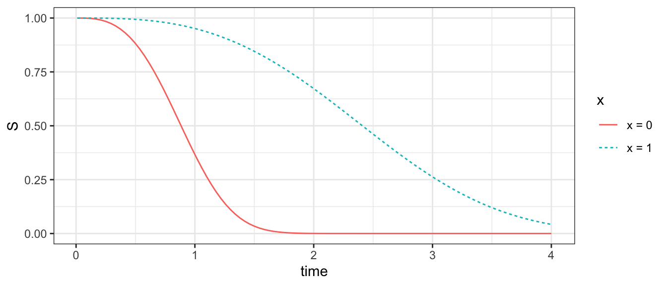
We can plot those survival curves!

predicted_survival |>
  # Make x a character for easier plotting
  mutate(x = paste("x =",x)) |>
  ggplot(aes(x = time, y = S, color = x, linetype = x)) +
  geom_line()

See differences from Exponential

You may wonder how your Weibull model differs from an Exponential model. The hazard may change over time in the Weibull, whereas it would be constant in the Exponential. We can see the Weibull result by predicting the hazard function,

predicted_hazard <- predicted_survival |>
  mutate(
    # Calculate the PDF at each point
    f = dweibull(x = time, shape = shape, scale = scale),
    # Hazard equals PDF over survival
    h = f / S
  )

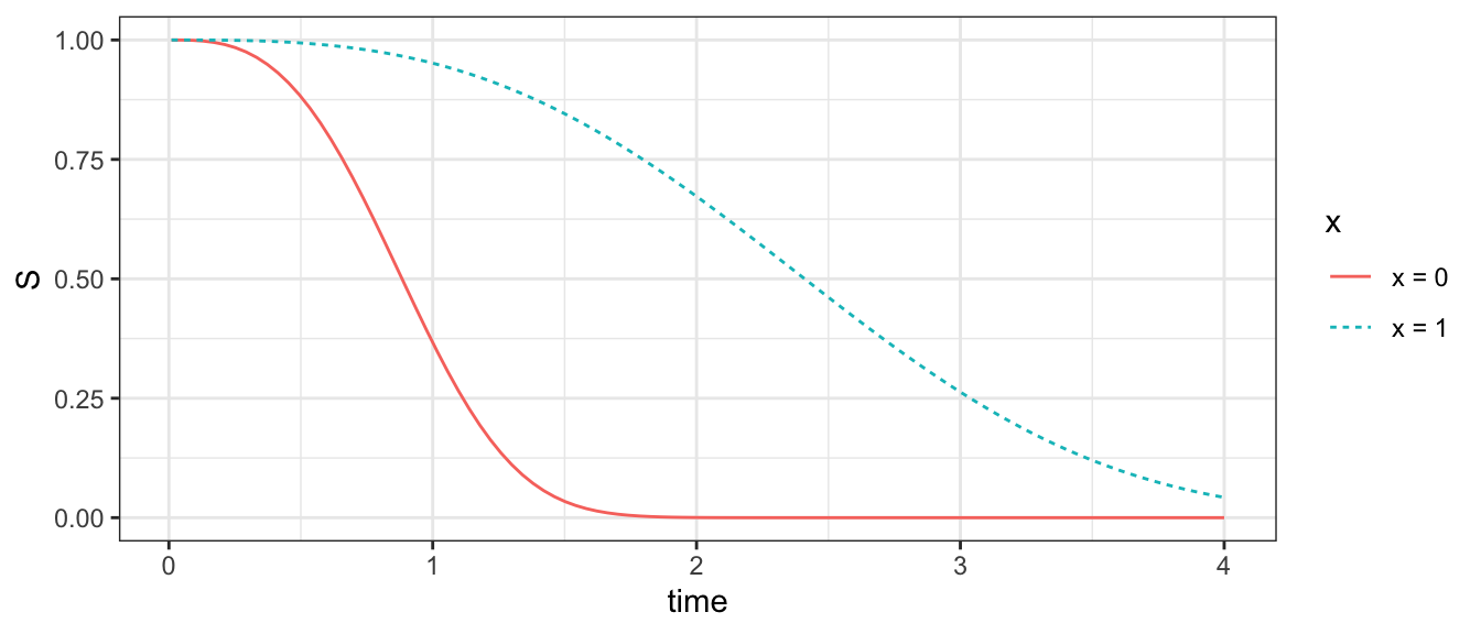
and plotting it as a function of time.

predicted_hazard |>
  # Make x a character for easier plotting
  mutate(x = paste("x =",x)) |>
  ggplot(aes(x = time, y = S, color = x, linetype = x)) +
  geom_line()

In this simulated example, the hazard function decreases with time.

To see the difference mathematically, note that the Weibull hazard wtih shape $\alpha$ and scale $\sigma$ is as follows. \[ h(t) = \alpha^{\alpha - 1}\sigma^{-\alpha}t^{\alpha - 1} \] Think about the particular case when $\alpha = 1$. Two of the exponents become 0 so that $\alpha^{\alpha - 1} = \alpha^0 = 1$ and $t^{\alpha - 1} = t^0 = 1$ and those terms drop out. The hazard becomes a constant function $\sigma^{-1}$. \[ h_{\alpha = 0}(t) = \sigma^{-1} \] This hazard is equivalent to an Exponential hazard, where $\sigma = \frac{1}{\lambda}$ with $\sigma$ the scale (larger for longer survival times) and $\lambda$ is the rate of events (larger for shorter survival times). Thus, the Weibull with $\alpha = 1$ is an exponential.

We might want to test to reject the null that $\alpha = 1$ in our Weibull model. Note that the shape parameter $\alpha$ is 1 / model$scale where model is a Weibull fitted with survreg and scale is what survreg calls the relevant parameter. The Exponential is thus the special case where model$scale = 1, or equivalently the log of the survreg scale parameter equals zero. There is a statistical test of this in the output of summary(model).

summary(model)


Call:
survreg(formula = Surv(t, 1 - c) ~ x, data = simulated, dist = "weibull")
               Value Std. Error       z      p
(Intercept) -0.00118    0.00485   -0.24   0.81
x            1.00311    0.00668  150.16 <2e-16
Log(scale)  -1.09656    0.00782 -140.22 <2e-16

Scale= 0.334 

Weibull distribution
Loglik(model)= -7894   Loglik(intercept only)= -13147.3
    Chisq= 10506.57 on 1 degrees of freedom, p= 0 
Number of Newton-Raphson Iterations: 6 
n= 10000

In this case, we can easily reject the null that Log(scale) equals 0. There is significant evidence that the Weibull fits the data better than the Exponential.

We might want a confidence interval on the $\alpha$ shape parameter. To do that, we first extract the log scale estimate and standard error from the survreg model.

log_scale_estimate <- log(model$scale)
log_scale_se <- sqrt(diag(model$var))["Log(scale)"]

Then, we use the Normal to construct a 95% confidence interval on the log scale parameter.

log_scale_ci_lower <- log_scale_estimate - log_scale_se * qnorm(.975)
log_scale_ci_upper <- log_scale_estimate + log_scale_se * qnorm(.975)

Finally, we convert: the scale parameter is the exponentiated log scale parameter, and the rweibull $\alpha$ parameter shape is the inverse of the survreg parameter scale. Thus, we convert everything by the function $1 / \exp(x)$.

c(
  shape_estimate = 1 / exp(log_scale_estimate),
  ci_lower = 1 / exp(log_scale_ci_upper) |> unname(),
  ci_upper = 1 / exp(log_scale_ci_lower) |> unname()
)

shape_estimate       ci_lower       ci_upper 
      2.993838       2.948300       3.040079

Exercise

Load the heart_recipients data.

heart_recipients <- read_csv("https://ilundberg.github.io/eventhistory/assets/heart_recipients.csv")

Estimate a Weibull model for survival time t since a heart transplant, using age at transplant as a predictor.

Pick two ages and plot the estimated survival functions.
Pick two ages and plot the estimated hazard functions.
Can you reject the null that your model is equivalent to an Exponential?