MSM with One Treatment Period

Marginal structural modeling is a general tool for estimating causal effects under selection on observables. A marginal structural model (MSM) separates two steps:

• use weights to address confounding
• use a model for \(Y^a\) to pool information across treatment values

This page introduces this idea with a focus on survival outcome modeling for time-to-event data in the presence of ignorable censoring.

Concept of weighting

Consider a person \(i\) who receives treatment with probability \(\text{P}(A = 1\mid \vec{X} = \vec{x}_i) = 20\%\). We can think about 5 people who are observationally identical to person \(i\) (with \(\vec{X} = \vec{x}_i\)). The 20% probability means that in expectation one of these people is treated and 4 others are not. If person \(i\) is treated, we might say they represent a total of 5 people. We could calculate that probability by taking the inverse of the probability of treatment: \(\frac{1}{0.2} = 5\). This is the intuition of inverse probability of treatment weighting.

More generally, define a function that takes a treatment value \(a\) and confounder vector \(\vec{x}\) and returns an inverse probability of treatment weight.

\[ w(a,\vec{x}) = \frac{1}{\text{P}(A = a \mid\vec{X} = \vec{x})} \]

The weight \(w(a,\vec{x})\) answers the question: if I see a person \(i\) with \(A_i = a\) and I want to study a counterfactual pseudo-population in which everyone receives treatment value \(a\), how many people does person \(i\) represent?

Sample estimator by weighting

For average potential outcomes in the absence of censoring, the weight function yields a weighting estimator,

\[ \hat{\text{E}}\left(Y^a\right) = \frac{\sum_{i:A_i=a} Y_i w(A_i,\vec{X}_i)}{\sum_{i:A_i=a}w(A_i,\vec{X}_i)} \]

which is the weighted sample mean of \(Y_i\) among the units with \(A_i = a\).

Weighting for survival outcomes

For survival outcomes, the formula above may not be useful because there exists censoring. If \(Y\) is time to (event) and \(\tilde{Y}\leq Y\) is time to (event or censoring), then any summary of the observable \(\tilde{Y}\) will be downwardly biased for the corresponding summary of event times \(Y\). This is why we need a survival model.

Marginal structural models (Hernan et al. 2001) generalize the weighting idea to settings where an outcome model is necessary. The approach proceeds in several steps:

1. Model treatment assignment \(\text{P}(A\mid\vec{X})\)
2. Construct inverse probability of treatment weights \(w(A_i,\vec{X}_i)\) for each \(i\)
   • Note that the treatment value \(A_i\) is whatever treatment value was observed for unit \(i\)
3. Model the outcome \(Y_i\) as a function of \(A_i\), weighted by \(w(A_i,\vec{X}_i)\)
4. Predict quantities of interest

Worked example

Try sketching out these steps for the veteran example before looking at the code below.

1. Model treatment assignment \(\text{P}(A\mid\vec{X})\)

model_treatment <- glm(
  I(trt == 2) ~ karno + diagtime + age + prior,
  data = veteran,
  family = binomial()
)

2. Construct weights by the inverse probability of treatment
   • Note that the treatment value \(A_i\) is whatever treatment value was observed for unit \(i\)

weighted <- veteran |>
  mutate(
    p_treated = predict(model_treatment, type = "response"),
    p_control = 1 - p_treated,
    weight = case_when(
      trt == 1 ~ 1 / p_control,
      trt == 2 ~ 1 / p_treated
    )
  )

3. Model outcome values \(Y_i\) as a function of \(A_i\), weighted by \(w(A_i,\vec{X}_i)\). This is your marginal structural model.

model_outcome <- survreg(
  Surv(time, status) ~ trt,
  data = weighted,
  weights = weight
)

model_outcome_km <- survfit(
  Surv(time, status) ~ trt,
  data = weighted,
  weights = weight
)

4. Predict quantities of interest from your marginal structural model.

Note that because the MSM has already marginalized over \(\vec{X}\), the data to predict are only the treatment values of interest.

to_predict <- tibble(trt = 1:2)

How would you write code to predict some survival quantity from your marginal structural model? Sketch a plan before looking at the example code.

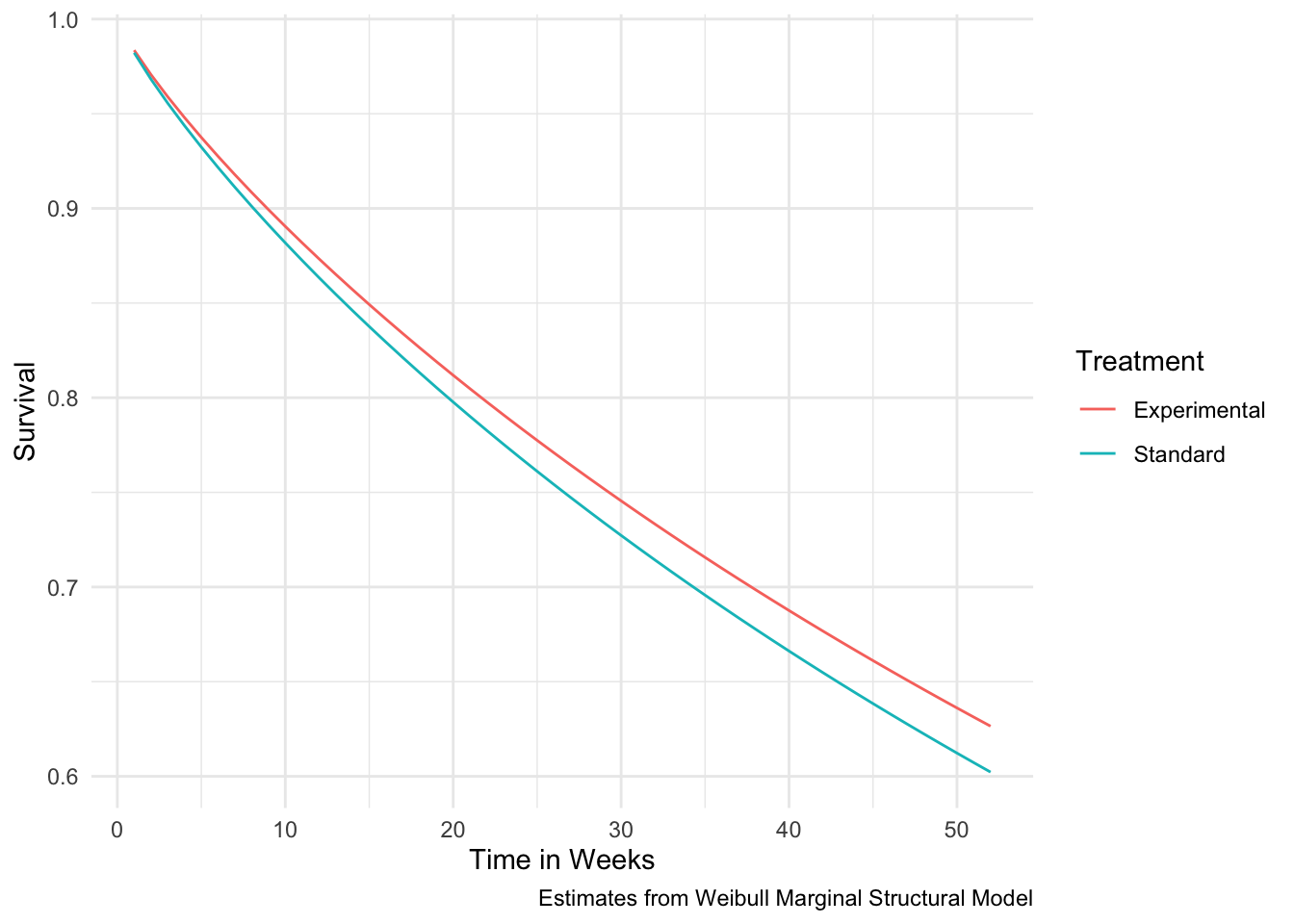
# This example code generates survival curves over the first year.

# Predict the shape and scale at each treatment value
predicted <- to_predict |>
  mutate(
    shape = 1 / model_outcome$scale,
    xb = predict(
      model_outcome, 
      newdata = to_predict, 
      type = "linear"
    )
  ) |>
  # Expand to predict for week 1 to 52
  uncount(weights = 52) |>
  mutate(time = rep(1:52, 2)) |>
  # Calculate survival probabilities
  mutate(
    survival = pweibull(
      time, 
      shape = shape, 
      scale = exp(xb), 
      lower.tail = FALSE
    )
  )

# Make a graph
predicted |>
  # Modify treatment to make plot easier to read
  mutate(
    trt = factor(trt, labels = c("Standard","Experimental")),
    trt = fct_rev(trt)
  ) |>
  ggplot(aes(x = time, y = survival, color = trt)) +
  geom_line() +
  labs(
    x = "Time in Weeks", 
    y = "Survival", 
    color = "Treatment",
    caption = "Estimates from Weibull Marginal Structural Model"
  )

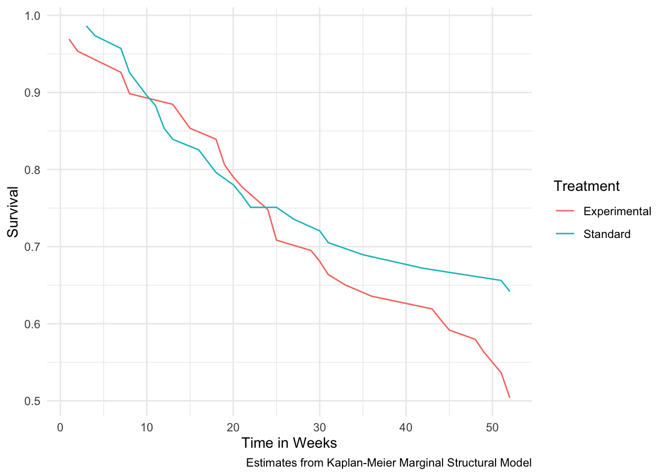
model_outcome_km |>
  broom::tidy() |>
  # Modify treatment to make plot easier to read
  mutate(
    strata = case_when(
      strata == "trt=1" ~ "Standard",
      strata == "trt=2" ~ "Experimental"
    )
  ) |>
  filter(time <= 52) |>
  ggplot(aes(x = time, y = estimate, color = strata)) +
  geom_line() +
  labs(
    x = "Time in Weeks", 
    y = "Survival", 
    color = "Treatment",
    caption = "Estimates from Kaplan-Meier Marginal Structural Model"
  )